Applied numerical modeling of saturated / unsaturated flow and ...

276
S. Bauer et al.
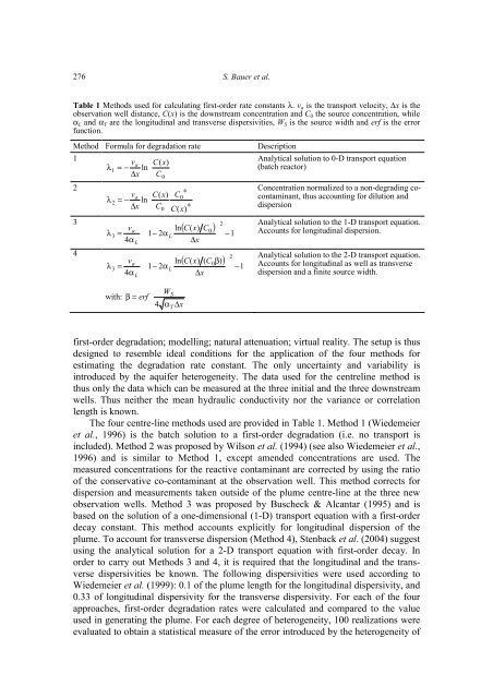
Table 1 Methods used for calculating first-order rate constants λ. va is the transport velocity, ∆x is the
observation well distance, C(x) is the downstream concentration and C0 the source concentration, while
αL and αT are the longitudinal and transverse dispersivities, WS is the source width and erf is the error
function.
Method Formula for degradation rate Description
1
va � C(
x)
�
λ1
= − ln� �
∆x
� �
� C0
�
Analytical solution to 0-D transport equation
(batch reactor)
2
v � ∗ �
a � C(
x)
C0
λ = −
�
2 ln
∆x
� C ∗ �
� 0 C(
x)
�
Concentration normalized to a non-degrading cocontaminant,
thus accounting for dilution and
dispersion
3
�
2
v
( ) �
a ��
ln C(
x)
C0
�
λ = � − α
� −1�
3 1 2 L
4α
�
�
L ��
∆x
� �
Analytical solution to the 1-D transport equation.
Accounts for longitudinal dispersion.
4
�
2
v
( ) �
a ��
ln C(
x)
( C0β)
�
λ = � − α
� −1�
3 1 2 L
4α
�
�
L ��
∆x
� �
Analytical solution to the 2-D transport equation.
Accounts for longitudinal as well as transverse
dispersion and a finite source width.
� �
with: � WS
β = erf �
� �
� 4 αT
∆x
�
first-order degradation; modelling; natural attenuation; virtual reality. The setup is thus
designed to resemble ideal conditions for the application of the four methods for
estimating the degradation rate constant. The only uncertainty and variability is
introduced by the aquifer heterogeneity. The data used for the centreline method is
thus only the data which can be measured at the three initial and the three downstream
wells. Thus neither the mean hydraulic conductivity nor the variance or correlation
length is known.
The four centre-line methods used are provided in Table 1. Method 1 (Wiedemeier
et al., 1996) is the batch solution to a first-order degradation (i.e. no transport is
included). Method 2 was proposed by Wilson et al. (1994) (see also Wiedemeier et al.,
1996) and is similar to Method 1, except amended concentrations are used. The
measured concentrations for the reactive contaminant are corrected by using the ratio
of the conservative co-contaminant at the observation well. This method corrects for
dispersion and measurements taken outside of the plume centre-line at the three new
observation wells. Method 3 was proposed by Buscheck & Alcantar (1995) and is
based on the solution of a one-dimensional (1-D) transport equation with a first-order
decay constant. This method accounts explicitly for longitudinal dispersion of the
plume. To account for transverse dispersion (Method 4), Stenback et al. (2004) suggest
using the analytical solution for a 2-D transport equation with first-order decay. In
order to carry out Methods 3 and 4, it is required that the longitudinal and the transverse
dispersivities be known. The following dispersivities were used according to
Wiedemeier et al. (1999): 0.1 of the plume length for the longitudinal dispersivity, and
0.33 of longitudinal dispersivity for the transverse dispersivity. For each of the four
approaches, first-order degradation rates were calculated and compared to the value
used in generating the plume. For each degree of heterogeneity, 100 realizations were
evaluated to obtain a statistical measure of the error introduced by the heterogeneity of