Applied numerical modeling of saturated / unsaturated flow and ...

More documents

Recommendations

Info

where vmax [s -1 ] is a maximum growth rate, Ci [kg m -3 ] is the concentration of the i th substrate, MCi [kg m -3 ] is the corresponding half velocity concentration [kg m -3 ], Cj [kg m -3 ] is the concentration of the j th substance inhibiting microbial growth, ICj is the corresponding inhibition concentration [kg m -3 ] and �(X) is a microbial decay term, which is often modeled as being of first order. Consumption of substrates or production of k metabolites Ck [kg m -3 ] is both coupled to microbial growth via (Schäfer et al., 1998) �Ck �1 ��X � � �t Y � � �t � � 6 (21) k growth where Yk [-] is the yield coefficient for substrate or metabolite Ck, and [·]growth refers to the growth term only in eq. (20). From the generalized Monod-type equation different more simple kinetic formulations can be derived. For a temporally constant microbial population, i.e. growth and decay terms are constant and of equal magnitude, no inhibition and dependence on only a single substrate, eq. (20) and (21) can be combined to yield the Michaelis-Menten (MM) kinetics model (Simkins and Alexander, 1984) dC dt C � �kmax (22) C � M C where k max is the maximum degradation rate [kg m -3 s -1 ] and M C is the MM half-saturation concentration [kg m -3 ]. This approximation may be applicable e.g. when aquifer sediments have been exposed to contaminants for several years (Bekins et al., 1998) and is used in application 2 (section 3.2). Often, contaminant degradation is also described by simple first order kinetics, e.g. to simulate abiotic degradation reactions like hydrolysis and dehydrohalogenation of halogenated compounds (Wiedemeier et al., 1999). First order kinetics can be derived from eq. (22) for C > MC eq. (22) approaches zero order kinetics. The first order model is used in application 1 and 3 (sections 3.1 and 3.3). Extensive reviews on kinetic models of biodegradation can be found e.g. in Baveye and Valocchi (1989), Rittmann and VanBriesen (1996) or Islam et al. (2001). 2.4. Numerics and software methods Numerical solution of the governing equations The governing equations for flow and reactive transport presented in sections 2.1 - 2.3 belong to the group of partial differential equations (PDE), containing derivatives of first order in time and of first as well as second order in space. The classification of PDE can be based on mathematical aspects (highest order derivatives in the dependent variables) or on a physical point of view (problem type of physical process) (Kolditz, 2002). Parabolic PDE are used for timedependent problems with dissipation process, such as diffusion (eq. (11)) or transient groundwater flow (eq. (3)), which convert to elliptic PDE for steady state conditions (eq. (4)). A third class of PDE are hyperbolic equations like the linear advection equation (eq. (10)), which are used to describe time-dependent problems without dissipation process. The transport equations (15) and (16) are of mixed type with a parabolic dispersion-diffusion term and a hyperbolic advection term. Their behaviour for a particular problem depends on the relative magnitudes of these flux components. In general the transport equations are of parabolic character which changes to hyperbolic for large ratios of v/�L as in this case the advective flux term is dominant (Kolditz, 2002). In general, PDE describing physical problems are well-posed when appropriate initial and boundary conditions are specified for the domain where a solution is required. While analytical solutions can be
found for a number of problems with simple geometries and boundary conditions (e.g. Bear, 1979; Van Genuchten and Alves, 1982; Kinzelbach, 1983), for complex nonlinear problems exact solutions may not exist and thus approximate numerical solutions must be obtained. 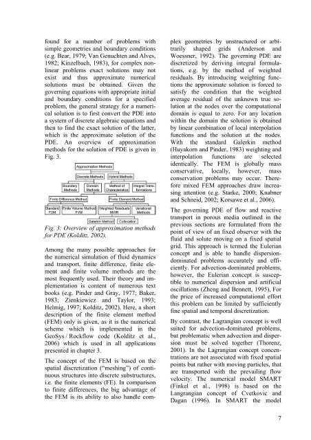Given the governing equations with appropriate initial and boundary conditions for a specified problem, the general strategy for a numerical solution is to first convert the PDE into a system of discrete algebraic equations and then to find the exact solution of the latter, which is the approximate solution of the PDE. An overview of approximation methods for the solution of PDE is given in Fig. 3. Fig. 3: Overview of approximation methods for PDE (Kolditz, 2002). Among the many possible approaches for the numerical simulation of fluid dynamics and transport, finite difference, finite element and finite volume methods are the most frequently used. Their theory and implementation is content of numerous text books (e.g. Pinder and Gray, 1977; Baker, 1983; Zienkiewicz and Taylor, 1993; Helmig, 1997; Kolditz, 2002). Here, a short description of the finite element method (FEM) only is given, as it is the numerical scheme which is implemented in the GeoSys / Rockflow code (Kolditz et al., 2006) which is used in all applications presented in chapter 3. The concept of the FEM is based on the spatial discretization (“meshing”) of continuous structures into discrete substructures, i.e. the finite elements (FE). In comparison to finite differences, the big advantage of the FEM is its ability to also handle complex geometries by unstructured or arbitrarily shaped grids (Anderson and Woessner, 1992). The governing PDE are discretized by deriving integral formulations, e.g. by the method of weighted residuals. By introducing weighting functions the approximate solution is forced to satisfy the condition that the weighted average residual of the unknown true solution at the nodes over the computational domain is equal to zero. For any location within the domain the solution is obtained by linear combination of local interpolation functions and the solution at the nodes. With the standard Galerkin method (Huyakorn and Pinder, 1983) weighting and interpolation functions are selected identically. The FEM is globally mass conservative, locally, however, mass conservation problems may occur. Therefore mixed FEM approaches draw increasing attention (e.g. Starke, 2000; Knabner and Schneid, 2002; Korsawe et al., 2006). The governing PDE of flow and reactive transport in porous media outlined in the previous sections are formulated from the point of view of an fixed observer with the fluid and solute moving on a fixed spatial grid. This approach is termed the Eulerian concept and is able to handle dispersiondominated problems accurately and efficiently. For advection-dominated problems, however, the Eulerian concept is susceptible to numerical dispersion and artificial oscillations (Zheng and Bennett, 1995), For the price of increased computational effort this problem can be limited by sufficiently fine spatial and temporal discretization. By contrast, the Lagrangian concept is well suited for advection-dominated problems, but problematic when advection and dispersion must be solved together (Thorenz, 2001). In the Lagrangian concept concentrations are not associated with fixed spatial points but rather with moving particles, that are transported with the prevailing flow velocity. The numerical model SMART (Finkel et al., 1998) is based on the Langrangian concept of Cvetkovic and Dagan (1996). In SMART the model 7
Page 3 and 4: Applied numerical modeling of satur
Page 5: Abstract Applied numerical modeling
Page 9: Vorwort Die zurückliegenden drei J
Page 13: List of abbreviations and mathemati
Page 16 and 17: for the application studies outline
Page 18 and 19: path lengths of water molecules tha
Page 22 and 23: domain is discretized along advecti
Page 24 and 25: conceptional model error: wrong pro
Page 26 and 27: The conceptual model used is a rigo
Page 28 and 29: equires therefore a higher degradat
Page 30 and 31: studied for heterogeneous sites wit
Page 32 and 33: Fig. 13: Plume length overestimatio
Page 34 and 35: concentration maximum is for the ca
Page 36 and 37: possibilities can not be provided n
Page 38 and 39: technischen Bauwerken. (Model based
Page 40 and 41: Schäfer, D., Dahmke, A., Kolditz,
Page 43: Enclosed Publication 1 Bauer, S., B
Page 46 and 47: Assessing measurements of first-ord
Page 55 and 56: WATER RESOURCES RESEARCH, VOL. 42,
Page 57 and 58: W01420 BAUER ET AL.: ASSESSING FIRS
Page 69: Enclosed Publication 3 Beyer, C., B
Page 72 and 73:
74 C. Beyer et al. / Journal of Con
Page 74 and 75:
Page 76 and 77:
Page 78 and 79:
Page 80 and 81:
Page 82 and 83:
Page 84 and 85:
Page 86 and 87:
Page 88 and 89:
Page 90 and 91:
Page 92 and 93:
Page 95:
Enclosed Publication 4 Bauer, S., B
Page 98 and 99:
Einführung In dieser Arbeit wird e
Page 100 and 101:
Entlang der so bestimmten Grundwass
Page 102 and 103:
Für die letztgenannten Methoden m
Page 104 and 105:
Um diesen Effekt zu verdeutlichen s
Page 106 and 107:
Unsicherheit zu. Für Methode 3 ( A
Page 108 and 109:
sagt sowie die zusätzliche Problem
Page 111:
Enclosed Publication 5 Beyer, C., C
Page 114 and 115:
(1995) yields a “hybrid” rate c
Page 116 and 117:
2 integral scale lY of 2.67 m and l
Page 118 and 119:
The approximate solution employed h
Page 120 and 121:
As Bauer et al. (2006a) demonstrate
Page 122 and 123:
Table 4: Normalized degradation rat
Page 124 and 125:
Comparing results for source widths
Page 127:
Enclosed Publication 6 Beyer, C., K
Page 130 and 131:
Einleitung und Zielsetzung In Deuts
Page 132 and 133:
die Anzahl Simulationsläufe den Vo
Page 134 and 135:
Grundlage des Korngrößenspektrums
Page 136 and 137:
Dies ist als konservative Abschätz
Page 138 and 139:
Randbedingungen abhängig ist. Aus
Page 140 and 141:
keinen Einfluss auf die abgebaute M
Page 142 and 143:
Carsell, R. F., Parish, R. S.: Deve
Page 144:
van Genuchten, M.T.: A closed form
show all

Applied numerical modeling of saturated / unsaturated flow and ...

You also want an ePaper? Increase the reach of your titles

Delete template?

Save as template?