Applied numerical modeling of saturated / unsaturated flow and ...

More documents

Recommendations

Info

2 integral scale lY of 2.67 m and ln-conductivity variance σ Y = 2.7 is used for the spatial correlation structure. Kef and lY 2 are taken from the Borden field site (Sudicky 1986), whereas the degree of heterogeneity σ Y was reported for the Columbus Air Force Base site (Rehfeldt et al. 1992). Porosity n is set to 0.33, resulting in va = 6.54 10 -7 m s -1 . For local dispersivities αL and αT values of 0.25 m and 0.05 m are used. The contaminant source introduced in the aquifers is of rectangular shape centered at [11.5 m; 32.0 m] downstream of the inflow boundary and has an area of either 3 * 4 m or 3 * 16 m, corresponding to a source width WS of 1.5 or 6 correlation lengths transverse to the mean flow direction. It emits a contaminant with the contaminant concentration fixed in the source area at C / C0 = 1.0. The dissolved contaminant is subject to a first order kinetics degradation reaction with a rate constant λ of 1.59·10 -8 s -1 (0.5 a -1 = 0.5 yr -1 ). This value is well within the range of reported / recommended first order degradation rate constants for chlorinated solvents as well as petroleum hydrocarbons under anaerobic conditions listed in Aronson and Howard (1997). The model parameters used are summarized in Table 1. 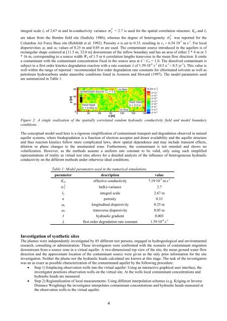contaminant source: C = 1.0 0 fixed head h = 0.552 m 4 no flow no flow fixed head h = 0.0 m -1 K [m s ] Figure 2: A single realization of the spatially correlated random hydraulic conductivity field and model boundary conditions. The conceptual model used here is a rigorous simplification of contaminant transport and degradation observed in natural aquifer systems, where biodegradation is a function of electron acceptor and donor availability and the aquifer structure and thus reaction kinetics follow more complicated laws, show spatial dependence and may include transient effects, dilution or phase changes to the unsaturated zone. Furthermore, the contaminant is not retarded and shows no volatilization. However, as the methods assume a uniform rate constant to be valid, only using such simplified representations of reality as virtual test sites allows for a detailed analysis of the influence of heterogeneous hydraulic conductivity on the different methods under otherwise ideal conditions. 1.0*10 -2 1.0*10 -3 1.0*10 -4 1.0*10 -5 1.0*10 -6 1.0*10 -7 1.0*10 -8 1.0*10 -9 Table 1: Model parameters used in the numerical simulations. parameter description value Kef effective conductivity 7.19·10 -5 m s -1 2 σ Y ln(K)-variance 2.7 lY integral scale 2.67 m n porosity 0.33 αL longitudinal dispersivity 0.25 m αT transverse dispersivity 0.05 m I hydraulic gradient 0.003 λ first order degradation rate constant 1.59·10 -8 s -1 Investigation of synthetic sites The plumes were independently investigated by 85 different test persons, engaged in hydrogeological and environmental research, consulting or administration. These investigators were confronted with the scenario of contaminant migration downstream from a source zone in a virtual aquifer. A two-dimensional top view of the site, the mean ground water flow direction and the approximate location of the contaminant source were given as the only prior information for the site investigation. Neither the plume nor the hydraulic heads calculated are known at this stage. The task of the investigators was an as exact as possible characterization of the contaminated aquifer by the following procedure: • Step 1) Emplacing observation wells into the virtual aquifer: Using an interactive graphical user interface, the investigator positions observation wells on the virtual site. At the wells local contaminant concentrations and hydraulic heads are measured. • Step 2) Regionalization of local measurements: Using different interpolation schemes (e.g. Kriging or Inverse Distance Weighting) the investigator interpolates contaminant concentrations and hydraulic heads measured at the observation wells to the virtual aquifer.
Steps 1 and 2 could be repeated as often as desired by the investigator, until the interpolated contaminant plume was deemed to be investigated accurately enough to properly characterize the contaminant distribution. Thus the interactive site investigation is an iterative procedure and is evaluated by a comparison of the “true” plume with the investigation result. More details on this procedure can be found in Chen et al. (2005). Using this methodology, a total number of 85 individual investigation results were obtained. 47 of these investigations were conducted for plumes originating from a source of width 4 m, while the plumes with a source width of 16 m were investigated 38 times. Accordingly, the majority of the 20 different plumes were investigated three or four times by different investigators. The configuration and the number of monitoring wells varies substantially between the different realizations and even for the same realization but different investigators (12 – 93 wells), as the decision about how many wells were needed for an accurate characterization of the site was left to the individual investigators. For two contaminant plumes (one for each source width) the investigation was repeated 13 times. Each investigation was performed by a different investigator. In addition to the general comparison of strategies A and B for the inference of the degradation rate constant, this subset of the whole data set allows for an analysis of estimated rate constant variability for a single site, resulting from different notions of “sufficient accuracy” of the virtual plume investigation. Rate constant estimation Using the monitoring networks installed by the investigators of the virtual plumes, first order rate constants were estimated following strategies A and B. Methods A1, A2 and A3 are used in strategy A and are described in detail in Bauer et al. (2006a). Therefore, only a brief description is given here: Method A1 (equation (3)) is based on the one-dimensional transport equation, considering advection and first order degradation only. The steady state solution for the concentration profile is rearranged to yield λA1, i.e. the first order degradation rate constant for method A1: va ⎛ C( x) ⎞ λ A1 = − ln⎜ ⎟ ∆x ⎜ ⎟ (3) ⎝ C0 ⎠ va [L T -1 ] is the transport velocity, ∆x [L] the distance between the observation wells and C0 and C(x) [M L -3 ] are upstream and downstream contaminant concentrations at the observation wells, respectively. λA1 can be considered rather an overall or bulk attenuation rate than a degradation rate constant (Newell et al. 2002), as all concentration changes due to diffusion, dispersion, volatilization or dilution are attributed to the degradation process. The method introduced by Buscheck and Alcantar (1995) is the second approach applied in this study (equation (4)). It is based on the steady state solution of the one-dimensional transport equation considering advection, longitudinal dispersion and first order degradation. Method A2 requires an estimate of longitudinal dispersivity αL [L] and yields a “hybrid” rate constant between a bulk attenuation and a pure biodegradation rate constant, as the effects of transverse dispersion are still reflected in the rate constant estimate λA2. ⎛ 2 v ( ) ⎞ a ⎜⎛ ln C( x) C0 ⎞ λ = ⎜1 − 2 ⎟ −1⎟ A2 α L 4α ⎜ ⎟ L ⎝⎝ ∆x ⎠ ⎠ (4) Zhang and Heathcote (2003) proposed modifications to the method of Buscheck and Alcantar (1995) to improve the estimation of λ with regard to transverse dispersion. Correction terms derived from analytical solutions to the two- and three-dimensional advection dispersion equations including first order decay are used to account for lateral spreading and the width of the source zone WS [L] in two and three dimensions, respectively. Therefore information about WS, αL and αT are required for this approach. Method A3 (equation (5)) is the two-dimensional form of the method by Zhang and Heathcote (2003) and yields the biodegradation rate constant estimate λA3: 2 v ⎛ ( ) ⎞ a ⎜⎛ ln C( x) ( C0β ) ⎞ ⎛ ⎞ λ = − ⎟ A3 ⎜ ⎜1− 2α L ⎟ 1 with ⎜ WS β = erf ⎟ (5) 4α ⎟ L ⎝⎝ ∆x ⎠ ⎜ ⎟ ⎠ ⎝ 4 αT ∆x ⎠ For evaluation strategy B, method B (equation (6)) is used, which corresponds to the approach of Stenback et al. (2004). An approximate solution for the steady state concentration distribution derived from the two-dimensional advectiondispersion equation with first order degradation (Domenico and Schwartz 1990) is fitted to measured concentrations: C ⎪⎧ ⎛ ⎞⎪⎫ ⎪ ⎧ ⎛ ⎞ ⎛ ⎞⎪ ⎫ 0 ⎛ x ⎞ ⎨ ⎜ + ⎟ ⎜ − ⎨ ⎜ 4λ ⎟⎬ − ⎟ ⎜ ⎟ Bα L 2y WS 2y WS C( x, y) = exp 1− 1+ erf erf ⎬ (6) 2 ⎪⎩ ⎝ 2α ⎠ ⎜ ⎟ ⎪⎭ ⎪⎩ ⎜ ⎟ ⎜ ⎟ L ⎝ va ⎠ ⎝ 4 αT x ⎠ ⎝ 4 αT x ⎠⎪⎭ 5
Page 3 and 4:
Applied numerical modeling of satur
Page 5:
Abstract Applied numerical modeling
Page 9:
Vorwort Die zurückliegenden drei J
Page 13:
List of abbreviations and mathemati
Page 16 and 17:
for the application studies outline
Page 18 and 19:
path lengths of water molecules tha
Page 20 and 21:
where vmax [s -1 ] is a maximum gro
Page 22 and 23:
domain is discretized along advecti
Page 24 and 25:
conceptional model error: wrong pro
Page 26 and 27:
The conceptual model used is a rigo
Page 28 and 29:
equires therefore a higher degradat
Page 30 and 31:
studied for heterogeneous sites wit
Page 32 and 33:
Fig. 13: Plume length overestimatio
Page 34 and 35:
concentration maximum is for the ca
Page 36 and 37:
possibilities can not be provided n
Page 38 and 39:
technischen Bauwerken. (Model based
Page 40 and 41:
Schäfer, D., Dahmke, A., Kolditz,
Page 43:
Enclosed Publication 1 Bauer, S., B
Page 46 and 47:
Assessing measurements of first-ord
Page 48 and 49:
Page 50 and 51:
Page 52 and 53:
Page 55 and 56:
WATER RESOURCES RESEARCH, VOL. 42,
Page 57 and 58:
W01420 BAUER ET AL.: ASSESSING FIRS
Page 59 and 60:
Page 61 and 62:
Page 63 and 64:
Page 65 and 66: W01420 BAUER ET AL.: ASSESSING FIRS
Page 67 and 68: W01420 BAUER ET AL.: ASSESSING FIRS
Page 69: Enclosed Publication 3 Beyer, C., B
Page 72 and 73: 74 C. Beyer et al. / Journal of Con
Page 95: Enclosed Publication 4 Bauer, S., B
Page 98 and 99: Einführung In dieser Arbeit wird e
Page 100 and 101: Entlang der so bestimmten Grundwass
Page 102 and 103: Für die letztgenannten Methoden m
Page 104 and 105: Um diesen Effekt zu verdeutlichen s
Page 106 and 107: Unsicherheit zu. Für Methode 3 ( A
Page 108 and 109: sagt sowie die zusätzliche Problem
Page 111: Enclosed Publication 5 Beyer, C., C
Page 114 and 115: (1995) yields a “hybrid” rate c
Page 118 and 119: The approximate solution employed h
Page 120 and 121: As Bauer et al. (2006a) demonstrate
Page 122 and 123: Table 4: Normalized degradation rat
Page 124 and 125: Comparing results for source widths
Page 127: Enclosed Publication 6 Beyer, C., K
Page 130 and 131: Einleitung und Zielsetzung In Deuts
Page 132 and 133: die Anzahl Simulationsläufe den Vo
Page 134 and 135: Grundlage des Korngrößenspektrums
Page 136 and 137: Dies ist als konservative Abschätz
Page 138 and 139: Randbedingungen abhängig ist. Aus
Page 140 and 141: keinen Einfluss auf die abgebaute M
Page 142 and 143: Carsell, R. F., Parish, R. S.: Deve
Page 144: van Genuchten, M.T.: A closed form
show all

Applied numerical modeling of saturated / unsaturated flow and ...

You also want an ePaper? Increase the reach of your titles

Delete template?

Save as template?