Applied numerical modeling of saturated / unsaturated flow and ...

80 C. Beyer et al. / Journal of Contaminant Hydrology 87 (2006) 73–95
below CPL. To define the plume length for this study, the 1% relative concentration contour line of
the contaminants is used, i.e. CPL=C(x)/C0=0.01.
4.3. Numerical Monte-Carlo simulations
To study the influence of heterogeneous hydraulic conductivity on the investigation results
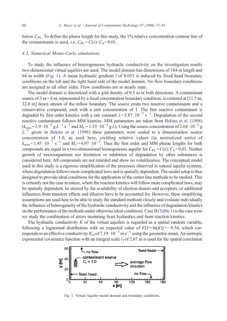
two-dimensional virtual aquifers are used. The model domain has dimensions of 184 m length and
64 m width (Fig. 1). A mean hydraulic gradient I of 0.053 is induced by fixed head boundary
conditions on the left and the right hand side of the model domain. No flow boundary conditions
are assigned to all other sides. Flow conditions are at steady state.
The model domain is discretized with a grid density of 0.5 m in both directions. A contaminant
source of 3 m×8 m, represented by a fixed concentration boundary condition, is centered at [11.5 m;
32.0 m] down stream of the inflow boundary. The source emits two reactive contaminants and a
conservative compound, each with a unit concentration of 1. The first reactive contaminant is
degraded by first order kinetics with a rate constant λ=5.87·10 −7 s −1 . Degradation of the second
reactive contaminant follows MM kinetics. MM parameters are taken from Bekins et al. (1998)
(kmax=3.9·10 −9 g L −1 s −1 and MC=1.33·10 −3 g L). Using the source concentration of 2.68·10 −2 g
L −1 given in Bekins et al. (1998) these parameters were scaled to a dimensionless source
concentration of 1.0, as used here, yielding relative values (in normalized units) of
kmax=1.45·10 −7 s −1 and MC=4.97·10 −2 . Thus the first order and MM plume lengths for both
compounds are equal in a two-dimensional homogeneous aquifer for CPL=C(x)/C0=0.01. Neither
growth of microorganisms nor limitation or inhibition of degradation by other substances is
considered here. All compounds are not retarded and show no volatilization. The conceptual model
used in this study is a rigorous simplification of the processes observed in natural aquifer systems,
where degradation follows more complicated laws and is spatially dependent. The model setup is thus
designed to provide ideal conditions for the application of the center line methods to be studied. This
is certainly not the case in nature, where the reaction kinetics will follow more complicated laws, may
be spatially dependent, be steered by the availability of electron donors and acceptors, or additional
influences from transient effects and dilution have to be accounted for. However, these simplifying
assumptions are used here to be able to study the standard methods closely and evaluate individually
the influence of heterogeneity of the hydraulic conductivity and the influence of degradation kinetics
on the performance of the methods under otherwise ideal conditions. Case B (Table 1) is the case were
we study the combination of errors stemming from hydraulics and from reaction kinetics.
The hydraulic conductivity K of the virtual aquifers is regarded as a spatial random variable,
following a lognormal distribution with an expected value of E[Y=ln(K)]=−9.54, which corresponds
to an effective conductivity Kef of 7.19·10 −5 ms −1 using the geometric mean. An isotropic
exponential covariance function with an integral scale lYof 2.67 m is used for the spatial correlation
Fig. 1. Virtual Aquifer model domain and boundary conditions.