Applied numerical modeling of saturated / unsaturated flow and ...

W01420 BAUER ET AL.: ASSESSING FIRST-ORDER RATES
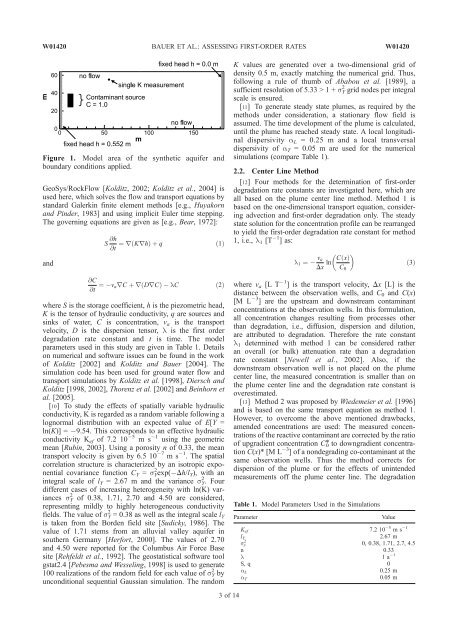
Figure 1. Model area of the synthetic aquifer and
boundary conditions applied.
GeoSys/RockFlow [Kolditz, 2002; Kolditz et al., 2004] is
used here, which solves the flow and transport equations by
standard Galerkin finite element methods [e.g., Huyakorn
and Pinder, 1983] and using implicit Euler time stepping.
The governing equations are given as [e.g., Bear, 1972]:
and
S @h
@t
¼rðKrhÞþq ð1Þ
@C
@t ¼ varC þrðDrCÞ lC ð2Þ
where S is the storage coefficient, h is the piezometric head,
K is the tensor of hydraulic conductivity, q are sources and
sinks of water, C is concentration, v a is the transport
velocity, D is the dispersion tensor, l is the first order
degradation rate constant and t is time. The model
parameters used in this study are given in Table 1. Details
on numerical and software issues can be found in the work
of Kolditz [2002] and Kolditz and Bauer [2004]. The
simulation code has been used for ground water flow and
transport simulations by Kolditz et al. [1998], Diersch and
Kolditz [1998, 2002], Thorenz et al. [2002] and Beinhorn et
al. [2005].
[10] To study the effects of spatially variable hydraulic
conductivity, K is regarded as a random variable following a
lognormal distribution with an expected value of E[Y =
ln(K)] = 9.54. This corresponds to an effective hydraulic
conductivity K ef of 7.2 10 5 ms 1 using the geometric
mean [Rubin, 2003]. Using a porosity n of 0.33, the mean
transport velocity is given by 6.5 10 7 ms 1 . The spatial
correlation structure is characterized by an isotropic exponential
covariance function C Y = s Y 2 exp( Dh/lY), with an
integral scale of l Y = 2.67 m and the variance s Y 2 . Four
different cases of increasing heterogeneity with ln(K) variances
s Y 2 of 0.38, 1.71, 2.70 and 4.50 are considered,
representing mildly to highly heterogeneous conductivity
fields. The value of s Y 2 = 0.38 as well as the integral scale lY
is taken from the Borden field site [Sudicky, 1986]. The
value of 1.71 stems from an alluvial valley aquifer in
southern Germany [Herfort, 2000]. The values of 2.70
and 4.50 were reported for the Columbus Air Force Base
site [Rehfeldt et al., 1992]. The geostatistical software tool
gstat2.4 [Pebesma and Wesseling, 1998] is used to generate
100 realizations of the random field for each value of s Y 2 by
unconditional sequential Gaussian simulation. The random
3of14
K values are generated over a two-dimensional grid of
density 0.5 m, exactly matching the numerical grid. Thus,
following a rule of thumb of Ababou et al. [1989], a
sufficient resolution of 5.33 > 1 + sY 2 grid nodes per integral
scale is ensured.
[11] To generate steady state plumes, as required by the
methods under consideration, a stationary flow field is
assumed. The time development of the plume is calculated,
until the plume has reached steady state. A local longitudinal
dispersivity aL = 0.25 m and a local transversal
dispersivity of aT = 0.05 m are used for the numerical
simulations (compare Table 1).
2.2. Center Line Method
[12] Four methods for the determination of first-order
degradation rate constants are investigated here, which are
all based on the plume center line method. Method 1 is
based on the one-dimensional transport equation, considering
advection and first-order degradation only. The steady
state solution for the concentration profile can be rearranged
to yield the first-order degradation rate constant for method
1, i.e., l 1 [T 1 ]as:
l1 ¼ va
Dx
Cx
ln ðÞ
C0
where va [L T 1 ] is the transport velocity, Dx [L] is the
distance between the observation wells, and C0 and C(x)
[M L 3 ] are the upstream and downstream contaminant
concentrations at the observation wells. In this formulation,
all concentration changes resulting from processes other
than degradation, i.e., diffusion, dispersion and dilution,
are attributed to degradation. Therefore the rate constant
l1 determined with method 1 can be considered rather
an overall (or bulk) attenuation rate than a degradation
rate constant [Newell et al., 2002]. Also, if the
downstream observation well is not placed on the plume
center line, the measured concentration is smaller than on
the plume center line and the degradation rate constant is
overestimated.
[13] Method 2 was proposed by Wiedemeier et al. [1996]
and is based on the same transport equation as method 1.
However, to overcome the above mentioned drawbacks,
amended concentrations are used: The measured concentrations
of the reactive contaminant are corrected by the ratio
of upgradient concentration C* 0 to downgradient concentration
C(x)* [M L 3 ] of a nondegrading co-contaminant at the
same observation wells. Thus the method corrects for
dispersion of the plume or for the effects of unintended
measurements off the plume center line. The degradation
Table 1. Model Parameters Used in the Simulations
Parameter Value
Kef 7.2 10 5 ms 1
lY sy
2.67 m
2
n
0, 0.38, 1.71, 2.7, 4.5
0.33
l 1a 1
S, q 0
aL 0.25 m
0.05 m
a T
W01420
ð3Þ