Applied numerical modeling of saturated / unsaturated flow and ...

More documents

Recommendations

Info

The approximate solution employed has the same basis as method 3. Here, however, a real two-dimensional approach is used, as equation (6) is fitted to the concentrations of all observation wells and not only to those measured along the center line. In strategy A the first step is an analysis of the concentration distribution based on all measurements made at the observation wells of the monitoring network. Starting at the well with the highest measured concentration, those downgradient wells are identified, that best represent the center line of the plume. These then are used to estimate the rate constant. Only locally measured quantities are used here, i.e. local hydraulic conductivities, hydraulic heads and contaminant concentrations are “measured” at these wells by reading the model data at the respective nodes of the numerical grid. The transport velocity va between each pair of center line wells is approximated by: ∆h va = K ef (7) n∆x with Kef the effective conductivity of local hydraulic conductivities at up and down gradient wells, n the porosity, ∆h the head difference and ∆x the distance between the wells. According to Rubin (2003) in stationary isotropic twodimensional domains with gaussian probability density functions of Y = ln(K) the effective conductivity Kef can be calculated as the geometric mean (cf. Bauer et al. 2006a). The porosity is assumed to be known correctly. With va, λ can then be calculated for each pair of center line wells using methods A1 – A3. For a set of k center line wells thus k-1 rate constants are calculated for one method. These are averaged to yield an estimate of the mean degradation rate constant λ. As an alternative to using only the locally measured conductivities, rate constant estimation is also performed using a global estimate of Kef, which is obtained from the geometric mean value of all hydraulic conductivities measured at all observation wells. In strategy B, method B (equation (6)) is fitted to measured concentrations of all observation wells of the monitoring network. Both the biodegradation rate constant λ and the source concentration C0 are varied simultaneously to achieve correspondence of measured and calculated concentrations, as a preliminary analysis (in agreement with results of Stenback et al. (2004)) showed that this procedure on average yields closer estimates of the true rate constant than fitting only λ with a single fixed estimate of the source concentration. A least squares criterion for the concentration residuals is used in the fitting procedure. As in strategy A the flow velocity va is approximated using equation (7). Kef is calculated as the geometric mean of hydraulic conductivities measured at all wells of the network. The average hydraulic gradient over the entire site is approximated by fitting a linear trend surface to all head measurements by ordinary least squares regression. For methods A2, A3 and B estimates of longitudinal and transverse dispersivities are required. Practical guidance on estimating these parameters at the field scale is given e.g. by Wiedemeier et al. (1999), where one suggestion is to use 0.1 times the plume length for αL and αT as 0.1 αL. Here, however, an alternative strategy is employed: Macrodispersivities 2 αL and αT are derived from correlation scale, aquifer heterogeneity σ Y and travel distance (Dagan 1984; Hsu 2003; Rubin et al. 2003). Thus, αL is taken as 7 m, which roughly corresponds to the large time asymptotic limit for the given conductivity distribution, while αT is taken as the approximate peak value of transverse macrodispersivity, calculated as 0.7 m (which thus also corresponds to the frequently used relationship as αT ≈ 0.1 αL). These values are well within the ranges of dispersivities commonly used for the field scale modeling of contaminant transport. The true value of the source width WS is assumed to be known from the site investigation. These approximations and assumptions were made to ensure that the error introduced in estimated rate constants due to the parameterization of methods A2, A3 and B is as small as possible. Results and Discussion Strategy A - One-dimensional center line approach The rate constants λA1 - λA3 estimated with equations (3) – (5) are divided by the “true” value used in the numerical simulations to yield normalized rate constants ΛA1 - ΛA3, which can directly be interpreted as overestimation or underestimation factors. Results in terms of mean values, medians, standard deviations and coefficients of variation (cv) as well as the number of realizations (N) used for strategy A are presented in Table 2 and Figure 3. Comparing methods A1 - A3 for the small source width WS = 4 m yields that all approaches on average result in a distinct overestimation of λ. For method A1 λ is overestimated on average by a factor of 6.88, while for A2 an mean ΛA2 = 8.24 is observed. Hence, method A1 performs better than A2. Method A3 yields a slightly lower mean of ΛA3 = 6.82, while the spread of results for A3 is noticeably larger, as can also be seen by the higher cv. Three main error sources for the observed overestimation exist: • neglect of dispersion by method A1, which thus is attributed to the degradation process (λA1 represents a bulk attenuation rate constant) 6
• deviation of sampling well locations from the true center line position, which causes the sampling of too low concentrations • unrepresentative estimates of the local va along the flow path, as the estimated λ increases and decreases with va (cf. equations (3) – (5)). These effects are discussed in detail in Bauer et al. (2006a). For method A2 the additional bias towards too large rate constants is a consequence of accounting only for αL in equation (4), as with a one-dimensional transport model longitudinal dispersion of a degrading contaminant results in a stronger spreading of the solute downstream and consequently in higher concentrations along the center line of a steady state plume compared to an advection only case. Therefore a larger rate constant is needed to fit a given concentration decrease and the “hybrid” rate constant estimate ΛA2 is always larger than the bulk attenuation rate constant ΛA1 (cf. Bauer et al. 2006a), which appears contradictory. Table 2: Normalized degradation rate constants estimated with strategy A. WS = 4 m method A1 method A2 method A3 mean 6.88 8.24 6.82 median 4.43 5.50 2.65 stdv. 6.36 7.41 10.09 cv 0.92 0.90 1.48 N 47 47 47 WS = 16 m method A1 method A2 method A3 mean 4.46 5.33 4.99 median 2.66 3.23 2.45 stdv. 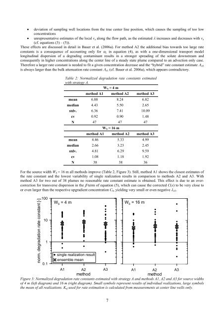4.81 6.29 9.59 cv 1.08 1.18 1.92 N 38 38 36 For the source width WS = 16 m all methods improve (Table 2, Figure 3). Still, method A1 shows the closest estimates of the rate constant and the lowest variability of single realization results in comparison to methods A2 and A3. With method A3 for two out of 38 plumes no reasonable rate constant estimate is obtained. This effect is due to an overcorrection for transverse dispersion in the β term of equation (5), which can cause the corrected C(x) to be very close to or even larger than the respective upgradient concentration C0, yielding very small or even negative λA3. norm. degradation rate constant [-] 100 10 1 W S = 4 m W S = 16 m single realization result ensemble mean 0.1 A1 1 A2 2 A3 3 A1 1 A2 2 A3 3 method method Figure 3: Normalized degradation rate constants estimated with strategy A and methods A1, A2 and A3 for source widths of 4 m (left diagram) and 16 m (right diagram). Small symbols represent results of individual realizations, large symbols the mean of all realizations. Kef used for rate estimation is calculated from measurements at center line wells only. 7
Page 3 and 4:
Applied numerical modeling of satur
Page 5:
Abstract Applied numerical modeling
Page 9:
Vorwort Die zurückliegenden drei J
Page 13:
List of abbreviations and mathemati
Page 16 and 17:
for the application studies outline
Page 18 and 19:
path lengths of water molecules tha
Page 20 and 21:
where vmax [s -1 ] is a maximum gro
Page 22 and 23:
domain is discretized along advecti
Page 24 and 25:
conceptional model error: wrong pro
Page 26 and 27:
The conceptual model used is a rigo
Page 28 and 29:
equires therefore a higher degradat
Page 30 and 31:
studied for heterogeneous sites wit
Page 32 and 33:
Fig. 13: Plume length overestimatio
Page 34 and 35:
concentration maximum is for the ca
Page 36 and 37:
possibilities can not be provided n
Page 38 and 39:
technischen Bauwerken. (Model based
Page 40 and 41:
Schäfer, D., Dahmke, A., Kolditz,
Page 43:
Enclosed Publication 1 Bauer, S., B
Page 46 and 47:
Assessing measurements of first-ord
Page 48 and 49:
Page 50 and 51:
Page 52 and 53:
Page 55 and 56:
WATER RESOURCES RESEARCH, VOL. 42,
Page 57 and 58:
W01420 BAUER ET AL.: ASSESSING FIRS
Page 59 and 60:
Page 61 and 62:
Page 63 and 64:
Page 65 and 66:
Page 67 and 68: W01420 BAUER ET AL.: ASSESSING FIRS
Page 69: Enclosed Publication 3 Beyer, C., B
Page 72 and 73: 74 C. Beyer et al. / Journal of Con
Page 95: Enclosed Publication 4 Bauer, S., B
Page 98 and 99: Einführung In dieser Arbeit wird e
Page 100 and 101: Entlang der so bestimmten Grundwass
Page 102 and 103: Für die letztgenannten Methoden m
Page 104 and 105: Um diesen Effekt zu verdeutlichen s
Page 106 and 107: Unsicherheit zu. Für Methode 3 ( A
Page 108 and 109: sagt sowie die zusätzliche Problem
Page 111: Enclosed Publication 5 Beyer, C., C
Page 114 and 115: (1995) yields a “hybrid” rate c
Page 116 and 117: 2 integral scale lY of 2.67 m and l
Page 120 and 121: As Bauer et al. (2006a) demonstrate
Page 122 and 123: Table 4: Normalized degradation rat
Page 124 and 125: Comparing results for source widths
Page 127: Enclosed Publication 6 Beyer, C., K
Page 130 and 131: Einleitung und Zielsetzung In Deuts
Page 132 and 133: die Anzahl Simulationsläufe den Vo
Page 134 and 135: Grundlage des Korngrößenspektrums
Page 136 and 137: Dies ist als konservative Abschätz
Page 138 and 139: Randbedingungen abhängig ist. Aus
Page 140 and 141: keinen Einfluss auf die abgebaute M
Page 142 and 143: Carsell, R. F., Parish, R. S.: Deve
Page 144: van Genuchten, M.T.: A closed form
show all

Applied numerical modeling of saturated / unsaturated flow and ...

Create successful ePaper yourself

Delete template?

Save as template?