Applied numerical modeling of saturated / unsaturated flow and ...

W01420 BAUER ET AL.: ASSESSING FIRST-ORDER RATES W01420
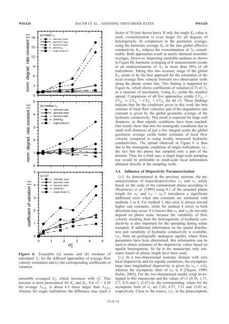
Figure 6. Ensemble (a) means and (b) medians of
calculated L 2 for the different approaches of average flow
velocity estimation and (c) the corresponding coefficients of
variation.
ensemble averaged L2, which increases with sY 2 . This
increase is most pronounced for Ka and KS. For sY 2 = 4.50
the average L2,K a is about 4.3 times larger than L2,K g ,
whereas for single realizations the difference may reach a
10 of 14
factor of 70 (not shown here). If only the single KS value is
used, overestimation is even larger for all degrees of
heterogeneity. In comparison to the geometric average,
using the harmonic average Kh or the true global effective
conductivity KG reduces the overestimation of L2 considerably.
Both approaches result in nearly identical ensemble
averages. However, inspecting ensemble medians as shown
in Figure 6b, harmonic averaging of K measurements results
in an underestimation of L2 in more than 50% of all
realizations. Taking this into account, usage of the global
KG seems to be the best approach for the estimation of the
local average flow velocity between two observation wells
along the plume center line. This finding is supported by
Figure 6c, which shows coefficients of variation (CV) ofL2
as a measure of uncertainty. Using KG yields the smallest
spread. Comparison of all five approaches yields: CVK G <
CVK g CVK h < CVK a < CVK S for all sY 2 . These findings
indicate that for the conditions given in this work the best
estimate of local flow velocities and of the degradation rate
constant is given by the global geometric average of the
hydraulic conductivity. This result is expected for large well
distances, as then ergodic conditions have been reached.
Our results show that also for nonergodic conditions due to
small well distances of just a few integral scales the global
geometric average yields better estimates of local flow
velocity compared to using locally measured hydraulic
conductivities. The spread observed in Figure 6 is thus
due to the nonergodic conditions of single realizations, i.e.,
the fact that the plume has sampled only a part of the
domain. Thus for a field case, a single large-scale pumping
test would be preferable to small-scale local information
obtained directly at the sampling wells.
3.4. Influence of Dispersivity Parameterization
[31] As demonstrated in the previous sections, the parameterization
of macrodispersivities a L and a T solely
based on the scale of the contaminant plume according to
Wiedemeier et al. [1999] using 0.1 of the assumed plume
length for a L and a T = a L/3 introduces a significant
additional error when rate constants are estimated with
methods 3 or 4. For method 3, this error is always toward
higher rate constants, while for method 4 errors in both
directions may occur. It is known that aL and aT do not only
depend on plume scale, because the variability of flow
velocity resulting from the heterogeneity of hydraulic conductivity
is also important for the spreading during solute
transport. If additional information on the spatial distribution
and variability of hydraulic conductivity is available,
i.e., from an geologically analogous aquifer, where these
parameters have been determined, this information can be
used to obtain estimates of the dispersivity values based on
aquifer heterogeneity. So far in the manuscript, only estimates
based on plume length have been used.
[32] In a two-dimensional isotropic domain with zero
local dispersivity and for ergodic conditions, the asymptotic
large time longitudinal dispersivity is given by aL = sY 2 lY,
whereas the asymptotic limit of aT is 0 [Dagan, 1989;
Rubin, 2003]. For the two-dimensional model setup investigated
in this manuscript and the values of sY 2 (0.38, 1,71,
2.7, 4.5) and lY (2.67) m, the corresponding values for the
asymptotic limit of aL are 1.02, 4.57, 7.21 and 12.02 m,
respectively. Close to the source, i.e., in the preasymptotic