Applied numerical modeling of saturated / unsaturated flow and ...

More documents

Recommendations

Info

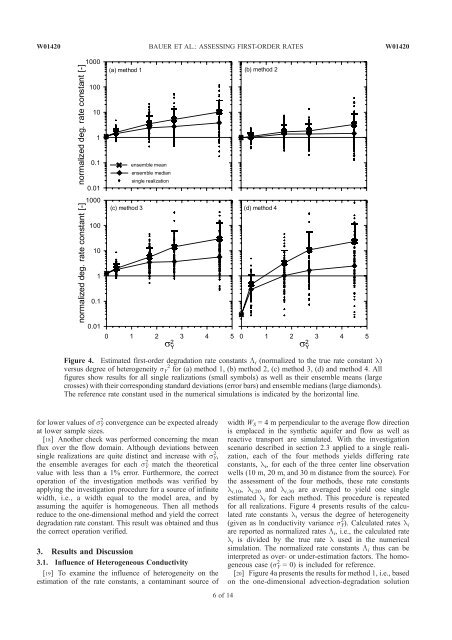
W01420 BAUER ET AL.: ASSESSING FIRST-ORDER RATES W01420 Figure 4. Estimated first-order degradation rate constants Li (normalized to the true rate constant l) versus degree of heterogeneity sY 2 for (a) method 1, (b) method 2, (c) method 3, (d) and method 4. All figures show results for all single realizations (small symbols) as well as their ensemble means (large crosses) with their corresponding standard deviations (error bars) and ensemble medians (large diamonds). The reference rate constant used in the numerical simulations is indicated by the horizontal line. for lower values of s Y 2 convergence can be expected already at lower sample sizes. [18] Another check was performed concerning the mean flux over the flow domain. Although deviations between single realizations are quite distinct and increase with s Y 2 , the ensemble averages for each s Y 2 match the theoretical value with less than a 1% error. Furthermore, the correct operation of the investigation methods was verified by applying the investigation procedure for a source of infinite width, i.e., a width equal to the model area, and by assuming the aquifer is homogeneous. Then all methods reduce to the one-dimensional method and yield the correct degradation rate constant. This result was obtained and thus the correct operation verified. 3. Results and Discussion 3.1. Influence of Heterogeneous Conductivity [19] To examine the influence of heterogeneity on the estimation of the rate constants, a contaminant source of 6of14 width W S = 4 m perpendicular to the average flow direction is emplaced in the synthetic aquifer and flow as well as reactive transport are simulated. With the investigation scenario described in section 2.3 applied to a single realization, each of the four methods yields differing rate constants, l i, for each of the three center line observation wells (10 m, 20 m, and 30 m distance from the source). For the assessment of the four methods, these rate constants l i,10, l i,20 and l i,30 are averaged to yield one single estimated l i for each method. This procedure is repeated for all realizations. Figure 4 presents results of the calculated rate constants l i versus the degree of heterogeneity (given as ln conductivity variance s Y 2 ). Calculated rates li are reported as normalized rates L i, i.e., the calculated rate l i is divided by the true rate l used in the numerical simulation. The normalized rate constants L i thus can be interpreted as over- or under-estimation factors. The homogeneous case (s Y 2 = 0) is included for reference. [20] Figure 4a presents the results for method 1, i.e., based on the one-dimensional advection-degradation solution
W01420 BAUER ET AL.: ASSESSING FIRST-ORDER RATES (equation (3)). It can be clearly seen, that an increase of sY 2 leads to an increase in spread of the single realizations. Quite a number of realizations exhibit normalized rate constants L1 of more than 10 up to about 100, i.e., the true rate constant is severely overestimated by a factor of 10 to 100. Also, L1 increases with increasing sY 2 as well as the standard deviations of the ensemble means. This points to an increase in uncertainty and reflects the spread of the single realizations. Mean overestimation increases from a factor of about 1.6 for sY 2 = 0.38 to about 10.2 in the case of sY 2 = 4.50. In the homogeneous case (sY 2 =0), method 1 yields the correct result. Although on average l is overestimated, even for high values of sY 2 in single realizations l may actually be underestimated by L1. For the highest degree of heterogeneity, the L1 of the single realizations span about three orders of magnitude. Comparison of ensemble means with the corresponding medians shows that in all cases the medians are significantly lower. The populations of estimated l1 are positively skewed as some exceedingly large values of l1 shift the means to high values. However, the general trend of increasing overestimation with heterogeneity is also distinct for the medians. [21] Figure 4b shows the corresponding results obtained with method 2, i.e., using the one dimensional advectiondegradation equation with normalization to a recalcitrant cocontaminant (equation (4)) [Wiedemeier et al., 1996]. As for method 1, the spread of the single realizations increases with increasing s Y 2 . Compared to method 1, however, the spread is smaller and more equally distributed about L 2 =1. Therefore the average overestimation factors as well as the standard deviations are much smaller than for method 1 and both the error and the uncertainty are lower. Average rate constants L 2 are 1.1 for s Y 2 = 0.38, increasing to 3.3 for sY 2 = 4.50. For homogeneous conditions, also method 2 yields the correct result, i.e., L 2 = 1 for s Y 2 = 0. Ensemble medians are just slightly above the true l, i.e., deviating less than a factor of 2. [22] Degradation rate constants calculated with method 3, i.e., the one-dimensional method introduced by Buscheck and Alcantar [1995] (equation (5)), are displayed in Figure 4c. They exhibit a similar general behavior as found with method 1, i.e., increasing spread and increasing overestimation of the true rate constant for higher s Y 2 . However, mean L3 are significantly higher than the corresponding L 1, with ensemble means of 2.0 for s Y 2 = 0.38 increasing to 29.4 for sY 2 = 4.50. In the homogeneous case, the true rate constant is slightly overestimated, i.e., L 3 =1.25fors Y 2 = 0. Spread in the single realizations is higher compared to method 1, now spanning nearly four orders of magnitude for the largest variance value of s Y 2 . [23] Results for method 4, i.e., the two-dimensional solution (equation (6)) suggested by Zhang and Heathcote [2003], are depicted in Figure 4d. Compared to the other methods, method 4 displays the largest spread of calculated L 4 around the mean values. For the highest degree of heterogeneity, the spread of the single realizations covers nearly five orders of magnitude. Ensemble means of L 4 increase from 0.6 for s Y 2 = 0.38 to about 23.0 for sY 2 = 4.5, i.e., for low s Y 2 the normalized rate constant L4 is actually underestimated in most realizations, while for larger varian- 7of14 W01420 ces the ensemble averages approach the results of method 3. In the homogeneous case (sY 2 = 0), the estimated rate constant l4 is about two orders of magnitude lower than the true rate constant l. Ensemble medians for method 4 show a similar behavior as the ensemble means, with their values closer to the true rate constant than for methods 1 and 3 for large heterogeneities (sY 2 = 1.71). This reflects the fact, that the spread of the single realizations is distributed symmetrically around L4 = 1, however, the spread of the populations and thus the uncertainty is significantly larger than for methods 1 and 3. [24] Method 1 is based on the one-dimensional solution to first-order biodegradation and advection. Therefore it is expected that rate constants estimated with method 1 overestimate the true rate constant due to two effects. Firstly, method 1 does not account for measuring off the center line. So if an observation well is placed off the plume center line, concentrations sampled there will be smaller than on the center line and therefore the degradation rate constant will be estimated too high. Secondly, as method 1 is based on a one-dimensional solution of the transport equation, it does not account for transverse dispersion, which lowers concentrations on the plume center line. This second effect also causes an overestimation of the rate constant. Both effects together cause the overestimation of the rate constant as shown in Figure 4a. Method 2 tries to overcome these two problems by normalization to a conservative tracer. Both above effects also determine the concentration of the nonreactive component, and are thus corrected for by the normalization. As is shown in Figure 4b, results of method 2 are considerably better than of method 1, both considering spread and ensemble averages. However, as can be seen from Figure 4b, method 2 does not correct for all effects, as overestimation is observed with increasing s Y 2 . Effects of dispersion and measuring off the center line are accounted for by method 2, so the deviation seen for method 2 has to have a hydraulic cause. This deviation is introduced by the determination of the average flow velocity between the observation wells, which is calculated using an averaged value of the hydraulic conductivity at the two observation wells. This averaged value may not be representative of the flow path between the two wells and bias may be introduced into the calculation of degradation rate constants. This effects is studied closely below in section 3.3. [25] Method 3 is based on the one-dimensional transport equation including advection, degradation and longitudinal dispersion. Results from method 3, as shown in Figure 4c, display a higher spread and higher ensemble averages compared to method 1. Because method 3 includes longitudinal dispersion, it should be closer to reality and advantageous over method 1. The differences in estimated rate constants between method 1 and 3 are therefore due to the longitudinal dispersivity a L in method 3. With the onedimensional transport model used, pronounced longitudinal dispersion of a degrading contaminant results in a stronger spreading of the solute downstream and thus in higher concentrations along the plume center line compared to an advection only case. Therefore a larger rate constant is calculated to accomplish a given concentration decrease between the upgradient and the downgradient observation well. l 3 grows linearly with a L and is always larger than l 1,
Page 3 and 4:
Applied numerical modeling of satur
Page 5:
Abstract Applied numerical modeling
Page 9: Vorwort Die zurückliegenden drei J
Page 13: List of abbreviations and mathemati
Page 16 and 17: for the application studies outline
Page 18 and 19: path lengths of water molecules tha
Page 20 and 21: where vmax [s -1 ] is a maximum gro
Page 22 and 23: domain is discretized along advecti
Page 24 and 25: conceptional model error: wrong pro
Page 26 and 27: The conceptual model used is a rigo
Page 28 and 29: equires therefore a higher degradat
Page 30 and 31: studied for heterogeneous sites wit
Page 32 and 33: Fig. 13: Plume length overestimatio
Page 34 and 35: concentration maximum is for the ca
Page 36 and 37: possibilities can not be provided n
Page 38 and 39: technischen Bauwerken. (Model based
Page 40 and 41: Schäfer, D., Dahmke, A., Kolditz,
Page 43: Enclosed Publication 1 Bauer, S., B
Page 46 and 47: Assessing measurements of first-ord
Page 55 and 56: WATER RESOURCES RESEARCH, VOL. 42,
Page 57 and 58: W01420 BAUER ET AL.: ASSESSING FIRS
Page 59: W01420 BAUER ET AL.: ASSESSING FIRS
Page 69: Enclosed Publication 3 Beyer, C., B
Page 72 and 73: 74 C. Beyer et al. / Journal of Con
Page 95: Enclosed Publication 4 Bauer, S., B
Page 98 and 99: Einführung In dieser Arbeit wird e
Page 100 and 101: Entlang der so bestimmten Grundwass
Page 102 and 103: Für die letztgenannten Methoden m
Page 104 and 105: Um diesen Effekt zu verdeutlichen s
Page 106 and 107: Unsicherheit zu. Für Methode 3 ( A
Page 108 and 109: sagt sowie die zusätzliche Problem
Page 111:
Enclosed Publication 5 Beyer, C., C
Page 114 and 115:
(1995) yields a “hybrid” rate c
Page 116 and 117:
2 integral scale lY of 2.67 m and l
Page 118 and 119:
The approximate solution employed h
Page 120 and 121:
As Bauer et al. (2006a) demonstrate
Page 122 and 123:
Table 4: Normalized degradation rat
Page 124 and 125:
Comparing results for source widths
Page 127:
Enclosed Publication 6 Beyer, C., K
Page 130 and 131:
Einleitung und Zielsetzung In Deuts
Page 132 and 133:
die Anzahl Simulationsläufe den Vo
Page 134 and 135:
Grundlage des Korngrößenspektrums
Page 136 and 137:
Dies ist als konservative Abschätz
Page 138 and 139:
Randbedingungen abhängig ist. Aus
Page 140 and 141:
keinen Einfluss auf die abgebaute M
Page 142 and 143:
Carsell, R. F., Parish, R. S.: Deve
Page 144:
van Genuchten, M.T.: A closed form
show all

Applied numerical modeling of saturated / unsaturated flow and ...

Create successful ePaper yourself

Delete template?

Save as template?