Applied numerical modeling of saturated / unsaturated flow and ...

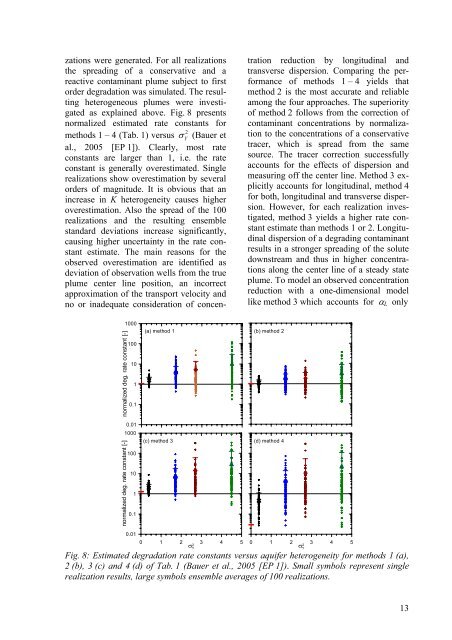
zations were generated. For all realizations
the spreading of a conservative and a
reactive contaminant plume subject to first
order degradation was simulated. The resulting
heterogeneous plumes were investigated
as explained above. Fig. 8 presents
normalized estimated rate constants for
2
methods 1 – 4 (Tab. 1) versus � Y (Bauer et
al., 2005 [EP 1]). Clearly, most rate
constants are larger than 1, i.e. the rate
constant is generally overestimated. Single
realizations show overestimation by several
orders of magnitude. It is obvious that an
increase in K heterogeneity causes higher
overestimation. Also the spread of the 100
realizations and the resulting ensemble
standard deviations increase significantly,
causing higher uncertainty in the rate constant
estimate. The main reasons for the
observed overestimation are identified as
deviation of observation wells from the true
plume center line position, an incorrect
approximation of the transport velocity and
no or inadequate consideration of concen-
normalized deg. rate constant [-]
normalized deg. rate constant [-]
1000
100
10
1
0.1
0.01
1000
100
10
1
0.1
0.01
(a) method 1 (b) method 2
(c) method 3 (d) method 4
0 1 2 3 4 5
tration reduction by longitudinal and
transverse dispersion. Comparing the performance
of methods 1 – 4 yields that
method 2 is the most accurate and reliable
among the four approaches. The superiority
of method 2 follows from the correction of
contaminant concentrations by normalization
to the concentrations of a conservative
tracer, which is spread from the same
source. The tracer correction successfully
accounts for the effects of dispersion and
measuring off the center line. Method 3 explicitly
accounts for longitudinal, method 4
for both, longitudinal and transverse dispersion.
However, for each realization investigated,
method 3 yields a higher rate constant
estimate than methods 1 or 2. Longitudinal
dispersion of a degrading contaminant
results in a stronger spreading of the solute
downstream and thus in higher concentrations
along the center line of a steady state
plume. To model an observed concentration
reduction with a one-dimensional model
like method 3 which accounts for �L only
0 1 2 3 4 5
�2 �2 Y Y
Fig. 8: Estimated degradation rate constants versus aquifer heterogeneity for methods 1 (a),
2 (b), 3 (c) and 4 (d) of Tab. 1 (Bauer et al., 2005 [EP 1]). Small symbols represent single
realization results, large symbols ensemble averages of 100 realizations.
13