Applied numerical modeling of saturated / unsaturated flow and ...

More documents

Recommendations

Info

W01420 BAUER ET AL.: ASSESSING FIRST-ORDER RATES W01420 rate constant for method 2 is then calculated as [Wiedemeier et al., 1996]: l2 ¼ va Dx Cx ln ðÞ C0 C* 0 C* ðÞ x A prerequisite for the application of method 2 is that physicochemical properties of degradable and recalcitrant compounds like Henry’s Law constants and sorption coefficients must be comparable. A group of substances that has been proven to be well suited for the normalization of downgradient concentrations in BTEX plumes under anaerobic conditions are several trimethylbenzene (TMB) isomers [EPA, 1998; Wiedemeier et al., 1996, 1999]. When TMB is subject to biodegradation the estimated rate constant will be less than the actual value. For chlorinated solvent plumes, inorganic compounds like chloride may be appropriate substances for the normalization. Reductive dechlorination results in the production of chloride along the flow path, which by means of a mass balance can be used to derive the correction factor [EPA, 1998]. [14] The third method investigated here was proposed by Buscheck and Alcantar [1995]. It is based on the steady state solution to the one-dimensional transport equation, accounting for advection, dispersion and first-order degradation. In comparison to method 1, method 3 accounts additionally for effects of longitudinal dispersion and thus requires an estimate of the longitudinal dispersivity aL [m]. The degradation rate constant for method 3 is given by Buscheck and Alcantar [1995]: l3 ¼ va ln 1 2aL 4aL Cx ðÞ 00 B C0 @@ Dx 1 A 2 1 ð4Þ C 1A ð5Þ Method 4 used here is the modified method of Buscheck and Alcantar [1995], as proposed by Zhang and Heathcote [2003]. Since in this study a two-dimensional synthetic aquifer is used to assess the different approaches, for method 4 the analytical solution to the two-dimensional transport equation including first order decay [Domenico, 1987] is adopted. Method 4 accounts for a finite source width as well as longitudinal and transverse dispersion. Therefore longitudinal and transverse dispersivities aL [m] and aT [m] as well as the source width WS [m] perpendicular to the average flow direction have to be known or estimated. Given these prerequisites, the degradation rate constant is given as [Zhang and Heathcote, 2003]: l4 ¼ va 1 4aL ln 2aL Cx ðÞ 00 B @@ C0b Dx b ¼ erf WS 1 A 2 1 C 1A 4 ffiffiffiffiffiffiffiffiffiffiffi p ð6Þ aT Dx 2.3. 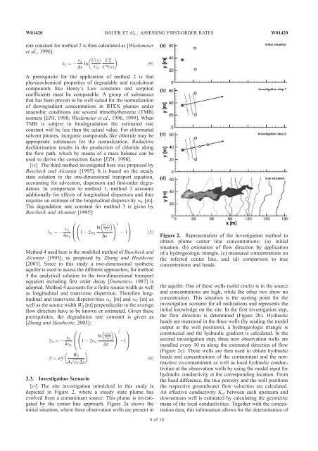Investigation Scenario [15] The site investigation mimicked in this study is depicted in Figure 2, where a steady state plume has evolved from a contaminant source. This plume is investigated by the center line approach. Figure 2a shows the initial situation, where three observation wells are present in 4of14 Figure 2. Representation of the investigation method to obtain plume center line concentrations: (a) initial situation, (b) estimation of flow direction by application of a hydrogeologic triangle, (c) measured concentrations on the inferred center line, and (d) comparison to true concentrations and heads. the aquifer. One of these wells (solid circle) is in the source and concentrations are high, while the other two show no concentration. This situation is the starting point for the investigation scenario for all realizations and represents the initial knowledge on the site. In the first investigation step, the flow direction is determined (Figure 2b). Hydraulic heads are measured in the three wells (by reading the model output at the well positions), a hydrogeologic triangle is constructed and the hydraulic gradient is calculated. In the second investigation step, three new observation wells are installed every 10 m along the estimated direction of flow (Figure 2c). These wells are then used to obtain hydraulic heads and concentrations of the contaminant and the nonreactive co-contaminant as well as local hydraulic conductivities at the observation wells by using the model input for hydraulic conductivity at the corresponding location. From the head difference, the true porosity and the well positions the respective groundwater flow velocities are calculated. An effective conductivity Kef between each upstream and downstream well is estimated by calculating the geometric mean of the local conductivities. Together with the concentration data, this information allows for the determination of
W01420 BAUER ET AL.: ASSESSING FIRST-ORDER RATES the first-order degradation rate constants by the four methods presented above. The investigation setup is designed to resemble ideal conditions for the application of the four methods for estimating the degradation rate constant. All measurements are assumed to be exact, which means that there is no measurement error involved. The only uncertainty and variability is introduced by the heterogeneity of hydraulic conductivity. For methods 3 and 4, additionally aL and aT have to be known. These are estimated following Wiedemeier et al. [1999] as 0.1 of the plume length for aL, with aT being about 0.33 of the longitudinal dispersivity. As plume length the maximum distance covered by the observation wells, i.e., 30 m, is used. As the plumes are generally longer, this assumption yields rather low dispersivities. Thus aL and aT are estimated to be 3.0 and 1.0 m, respectively. These estimates of dispersivities are not optimal, as they are not based on the heterogeneity of the hydraulic conductivity. However, dispersivities based on results from stochastic hydrogeology are difficult to obtain, as for most field sites structure and degree of heterogeneity are not well known. Also, the four samples taken in this investigation scenario do not allow for an estimation of the correlation length or the ln(K) variances. Both the correct source width and the correct porosity are used. In the last step, by each of the four approaches the corresponding first-order degradation rate constants l 1 through l 4 are calculated. These values can be compared to the value used to generate the plume (l =1a 1 ). For each realization, the investigation procedure described above is followed and a degradation rate is calculated for each method, each downstream well and for each source width. For each of the four classes of heterogeneity used in this study (ln(K) variances s Y 2 of 0.38, 1.71, 2.70 and 4.50) a minimum of 100 realizations is evaluated. Thus statistical measures of the errors and uncertainties introduced by the heterogeneity of the hydraulic conductivity are obtained. Additionally, also the impact of the width of the source zone is studied. Here it is expected, that for increasing source width the onedimensional methods yield better results, as then the investigated situation corresponds better to the assumptions of the method. Source widths W S of 4 m, 8 m and 16 m are used, corresponding to 1.5, 3 and 6 integral scales l Y. Then methods for estimating the flow velocity are elucidated for the different degrees of heterogeneity. This is because the goodness of the calculated value for lambda is directly related to estimated transport velocity accuracy. Finally the influence of estimated longitudinal and transversal dispersivities on results by methods 3 and 4 is studied in a sensitivity analysis. 2.4. Numerical Tests [16] Convergence of the Monte Carlo simulation with regard to the sample size N of estimated degradation rate constants was tested by a procedure following Goovaerts [1999]. The test is only conducted for the highest degree of heterogeneity used in this study (sY 2 = 4.5) and the smallest source width of 4 m, as this is the case of highest variability. A total of 1000 realizations of the random conductivity field was generated. For each realization, plume development was simulated and the degradation rate constant l1 was calculated using method 1. The resulting set of 1000 degradation rates is assumed to be sufficiently large to Figure 3. Influence of Monte Carlo sample size N on the average subset mean (l1), the standard deviation of subset means (sl1 ), and the average standard deviation of the subset population (sl1 ) for the highest degree of heterogeneity (sY 2 ). represent the global population. The global population of l1 was randomly sampled with a sample size of N =2, yielding a subset of two l1. For this subset the mean degradation rate as well as the standard deviation were calculated. Random sampling was repeated 999 times, resulting in 1000 subsets of N = 2. From these subsets, the average subset mean l1, the standard deviation of subset means sl1 and the average standard deviation of the subset population sl1 are calculated. Random sampling was repeated with increasing subset sizes N =3,4,..., 1000, resulting in 999 triplets of the statistics, one for each subset size. Dependence of the three statistics on N is shown in Figure 3. [17] The middle curve in Figure 3 displays the average subset mean l1, which shows almost no dependence on N and yields values very close to the global mean of 8.9. The standard deviation of the subset means (s , lower curve) l1 shows a strong decrease from 12.3 (N = 2) to 2.2 (N = 50) and 1.5 (N = 100), with a significantly reduced decrease for larger subset sizes. In relation to the global mean of 8.9, the variation among the subsets is therefore small for N 100. The upper curve in Figure 3 shows the average standard deviation of the random sample subsets sl1 , which strongly increases with subset size for small N, but with a much smaller increase for N > 50. For N = 100 a value of 15.5 is found, which is 95% of the standard deviation of the global population, as obtained for N = 1000. The observed reduction in increase of sl1 with N indicates the redundancy of additional realizations with regard to the subset variability. As the rate of decrease of s as well as the rate of increase l1 of sl1 becomes small for more than 100 realizations, we feel confident that a sample size of N = 100 is sufficient to yield stable ensemble averaged rate coefficients. Since the analysis was conducted for the largest degree of heterogeneity, 5of14 W01420
Page 3 and 4:
Applied numerical modeling of satur
Page 5:
Abstract Applied numerical modeling
Page 9: Vorwort Die zurückliegenden drei J
Page 13: List of abbreviations and mathemati
Page 16 and 17: for the application studies outline
Page 18 and 19: path lengths of water molecules tha
Page 20 and 21: where vmax [s -1 ] is a maximum gro
Page 22 and 23: domain is discretized along advecti
Page 24 and 25: conceptional model error: wrong pro
Page 26 and 27: The conceptual model used is a rigo
Page 28 and 29: equires therefore a higher degradat
Page 30 and 31: studied for heterogeneous sites wit
Page 32 and 33: Fig. 13: Plume length overestimatio
Page 34 and 35: concentration maximum is for the ca
Page 36 and 37: possibilities can not be provided n
Page 38 and 39: technischen Bauwerken. (Model based
Page 40 and 41: Schäfer, D., Dahmke, A., Kolditz,
Page 43: Enclosed Publication 1 Bauer, S., B
Page 46 and 47: Assessing measurements of first-ord
Page 55 and 56: WATER RESOURCES RESEARCH, VOL. 42,
Page 57: W01420 BAUER ET AL.: ASSESSING FIRS
Page 61 and 62: W01420 BAUER ET AL.: ASSESSING FIRS
Page 69: Enclosed Publication 3 Beyer, C., B
Page 72 and 73: 74 C. Beyer et al. / Journal of Con
Page 95: Enclosed Publication 4 Bauer, S., B
Page 98 and 99: Einführung In dieser Arbeit wird e
Page 100 and 101: Entlang der so bestimmten Grundwass
Page 102 and 103: Für die letztgenannten Methoden m
Page 104 and 105: Um diesen Effekt zu verdeutlichen s
Page 106 and 107: Unsicherheit zu. Für Methode 3 ( A
Page 108 and 109:
sagt sowie die zusätzliche Problem
Page 111:
Enclosed Publication 5 Beyer, C., C
Page 114 and 115:
(1995) yields a “hybrid” rate c
Page 116 and 117:
2 integral scale lY of 2.67 m and l
Page 118 and 119:
The approximate solution employed h
Page 120 and 121:
As Bauer et al. (2006a) demonstrate
Page 122 and 123:
Table 4: Normalized degradation rat
Page 124 and 125:
Comparing results for source widths
Page 127:
Enclosed Publication 6 Beyer, C., K
Page 130 and 131:
Einleitung und Zielsetzung In Deuts
Page 132 and 133:
die Anzahl Simulationsläufe den Vo
Page 134 and 135:
Grundlage des Korngrößenspektrums
Page 136 and 137:
Dies ist als konservative Abschätz
Page 138 and 139:
Randbedingungen abhängig ist. Aus
Page 140 and 141:
keinen Einfluss auf die abgebaute M
Page 142 and 143:
Carsell, R. F., Parish, R. S.: Deve
Page 144:
van Genuchten, M.T.: A closed form
show all

Applied numerical modeling of saturated / unsaturated flow and ...

You also want an ePaper? Increase the reach of your titles

Delete template?

Save as template?