Applied numerical modeling of saturated / unsaturated flow and ...

88 C. Beyer et al. / Journal of Contaminant Hydrology 87 (2006) 73–95
plume lengths only. The estimated contaminant plume lengths Li are displayed in Fig. 5 (single
realization results, ensemble means with standard deviations as error bars, medians, coefficients of
variation). As for case A, L1 and L2 (Fig. 5 (a)) yield very similar results. However, in comparison to
case A, underestimation is clearly increased. This is most obvious for homogeneous conditions, where
L1 and L2 are only about 50% of the true length and thus no longer yield the correct result.
Underestimation of L increases with heterogeneity, yielding mean values of L1 and L2 of 0.45 for
σ Y 2 =4.5. Spread is about 0.75 orders of magnitude for low heterogeneity and one order of magnitude
for high heterogeneities, which is similar to case A. Plume lengths L 3 (Fig. 5 (b)) show the same
general behaviour as the L1 and L2, with mean values being slightly lower. In contrast to this, L is
overestimated for most realizations by L4 (Fig. 5 (c)). While for homogeneous conditions a too short
L4 of 0.65 is obtained, L4 increases to values larger than one for higher degrees of heterogeneity.
Spread of single realizations is significantly increased in comparison to case A (compare Figs. 4 (c)
and 5(c)), as a spread of about one order of magnitude can be observed for all degrees of heterogeneity.
The additional error introduced by using methods 1 through 4 for plumes following Michaelis–
Menten kinetics degradation is most pronounced for low heterogeneities. Compared to case A,
plume lengths are underestimated to a larger extent, as can be seen by the lower mean values and
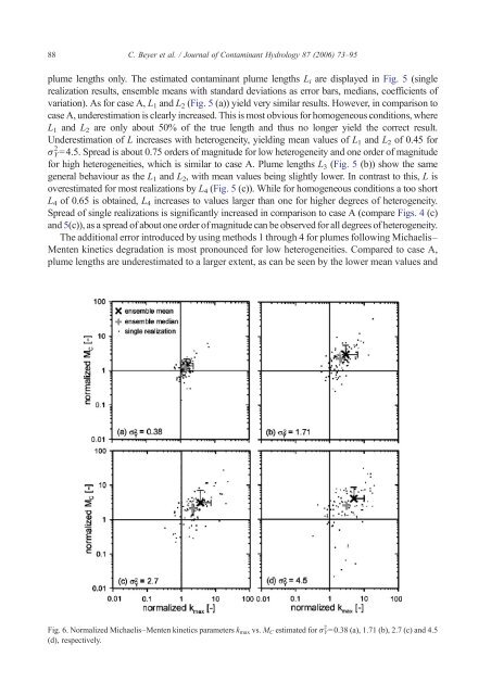
Fig. 6. Normalized Michaelis–Menten kinetics parameters kmax vs. MC estimated for σY 2 =0.38 (a), 1.71 (b), 2.7 (c) and 4.5
(d), respectively.