

Applied numerical modeling of saturated / unsaturated flow and ...
Applied numerical modeling of saturated / unsaturated flow and ...
Applied numerical modeling of saturated / unsaturated flow and ...

Create successful ePaper yourself
Turn your PDF publications into a flip-book with our unique Google optimized e-Paper software.
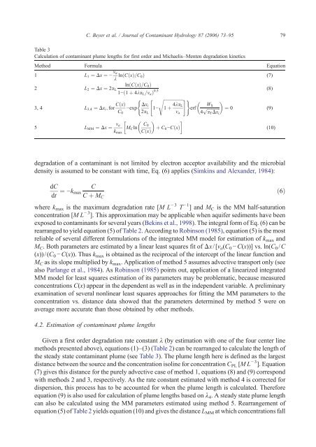
Table 3<br />
Calculation <strong>of</strong> contaminant plume lengths for first order <strong>and</strong> Michaelis–Menten degradation kinetics<br />
Method Formula Equation<br />
1 L1 ¼ Dx ¼ − va<br />
k lnðCðxÞ=C0Þ (7)<br />
2<br />
lnðCðxÞ=C0Þ<br />
L2 ¼ Dx ¼ 2aL<br />
1−ð1 þ 4kaL=vaÞ 0:5<br />
( " sffiffiffiffiffiffiffiffiffiffiffiffiffiffiffiffiffiffi#<br />
)<br />
(8)<br />
3, 4 L3;4 ¼ Dxi; for CðxÞ<br />
5 LMM ¼ Dx ¼ va<br />
degradation <strong>of</strong> a contaminant is not limited by electron acceptor availability <strong>and</strong> the microbial<br />
density is assumed to be constant with time, Eq. (6) applies (Simkins <strong>and</strong> Alex<strong>and</strong>er, 1984):<br />
dC<br />
dt<br />
C<br />
¼ −kmax<br />
C þ MC<br />
C. Beyer et al. / Journal <strong>of</strong> Contaminant Hydrology 87 (2006) 73–95<br />
where kmax is the maximum degradation rate [M L − 3 T − 1 ] <strong>and</strong> MC is the MM half-saturation<br />
concentration [ML − 3 ]. This approximation may be applicable when aquifer sediments have been<br />
exposed to contaminants for several years (Bekins et al., 1998). The integral form <strong>of</strong> Eq. (6) can be<br />
rearranged to yield equation (5) <strong>of</strong> Table 2. According to Robinson (1985), equation (5) is the most<br />
reliable <strong>of</strong> several different formulations <strong>of</strong> the integrated MM model for estimation <strong>of</strong> kmax <strong>and</strong><br />
MC. Both parameters are estimated by a linear least squares fit <strong>of</strong> Δx/[va(C0−C(x))] vs. ln(C0/C<br />
(x))/(C0−C(x)). Thus kmax is obtained as the reciprocal <strong>of</strong> the intercept <strong>of</strong> the linear function <strong>and</strong><br />
MC as its slope multiplied by kmax. Application <strong>of</strong> method 5 assumes advective transport only (see<br />
also Parlange et al., 1984). As Robinson (1985) points out, application <strong>of</strong> a linearized integrated<br />
MM model for least squares estimation <strong>of</strong> its parameters may be problematic, because measured<br />
concentrations C(x) appear in the dependent as well as in the independent variable. A preliminary<br />
examination <strong>of</strong> several nonlinear least squares approaches for fitting the MM parameters to the<br />
concentration vs. distance data showed that the parameters determined by method 5 were on<br />
average more accurate than those obtained by other methods.<br />
4.2. Estimation <strong>of</strong> contaminant plume lengths<br />
C0<br />
kmax<br />
−exp Dxi<br />
2aL<br />
1−<br />
1 þ 4kaL<br />
va<br />
Given a first order degradation rate constant λ (by estimation with one <strong>of</strong> the four center line<br />
methods presented above), equations (1)–(3) (Table 2) can be rearranged to calculate the length <strong>of</strong><br />
the steady state contaminant plume (see Table 3). The plume length here is defined as the largest<br />
distance between the source <strong>and</strong> the concentration isoline for concentration CPL [ML − 3 ]. Equation<br />
(7) gives this distance for the purely advective case <strong>of</strong> method 1, equations (8) <strong>and</strong> (9) correspond<br />
with methods 2 <strong>and</strong> 3, respectively. As the rate constant estimated with method 4 is corrected for<br />
dispersion, this process has to be accounted for when the plume length is calculated. Therefore<br />
equation (9) is also used for calculation <strong>of</strong> plume lengths based on λ4. A steady state plume length<br />
can also be calculated using the MM parameters estimated using method 5. Rearrangement <strong>of</strong><br />
equation (5) <strong>of</strong> Table 2 yields equation (10) <strong>and</strong> gives the distance L MM at which concentrations fall<br />
erf<br />
WS<br />
4 ffiffiffiffiffiffiffiffiffiffiffi p ¼ 0 (9)<br />
aTDxi<br />
MCln C0<br />
CðxÞ þ C0−CðxÞ (10)<br />
79<br />
ð6Þ


