Applied numerical modeling of saturated / unsaturated flow and ...

More documents

Recommendations

Info

conceptional model error: wrong process description 10 measurement error resulting investigation error conceptual site model investigation virtual aquifer Fig. 5: Virtual aquifer concept and possible sources of investigation error. An application of the VA concept requires the definition of a synthetic site model and its translation into a numerical model for the simulation of the identified relevant processes. Synthetic site models are generated based on statistical properties of natural aquifers. A defined contaminant source is then introduced and the evolution of aquifer contamination is simulated by numerical modeling, thus generating a realistic contaminant distribution in the synthetic aquifer. In comparison to the "real world", the unique advantage of the synthetic aquifer is that the spatial distribution of all physical and geochemical properties and parameters as well as contaminant concentrations are exactly known. Once the synthetic contaminated aquifer is generated, it can be studied by standard monitoring and investigation techniques, e.g. by emplacement of observation wells. Although the parameter distribution of the synthetic aquifer is known a priori, only the data “measured” at wells (i.e. hydraulic heads or concentrations) are used and interpreted. This is done because in a real site investigation also only a limited amount of measured data would be available. Finally, the results are compared to the “true” parameter distribution known from the synthetic aquifer, allowing an evaluation of the accuracy of the investigation method used. Using the VA concept, sources of uncertainty or error can be considered individually and the heterogeneity: incomplete or wrong description of parameter distribution sensitivity of investigation results on these can be studied. Stochastic approaches like the Monte-Carlo method are applied to study the propagation of parameter variability and uncertainty into the investigation results. The VA has been first introduced by Schäfer et al. (2002) and was applied by Schäfer et al. (2004, 2006b), Bauer and Kolditz (2006), Bauer et al. (2005 [EP 1]; 2006a [EP 2], 2007 [EP 4]) and Beyer et al. (2006 [EP 3], 2007a [EP 5]). An overview of VA applications is given in Bauer et al. (2006b) and Schäfer et al. (2006a). Fig. 6: Virtual investigation of a heterogeneous contaminant plume by the center line method (Bauer et al., 2005 [EP 1]). The VA concept is used here to study errors and uncertainties in degradation rate constants estimated from data typically collected by site investigation with the so called
center line method (Fig. 6). This method is frequently used in field studies when natural attenuation is considered as a remediation alternative and is based on observation wells that are placed along the presumed center line of the contaminant plume. Influence of measurement errors The first aspect studied here is the influence of measurement errors in hydraulic heads on degradation rate constant estimates (Bauer et al., 2007 [EP 4]). The VA concept used in this study is based on a two dimensional conceptual model of the groundwater body using a homogeneous distribution of hydraulic conductivity K. The development of the contaminant plume originating from a rectangular source zone is simulated until steady state conditions are established. The numerical simulations are performed using the GeoSys / Rockflow code, which was introduced in the previous chapter. The contaminant is subject to a first order kinetics (eq. (23)) degradation reaction using a uniform degradation rate constant �. Additionally, a conservative tracer is emitted from the source zone. The contaminant plume thus generated is then investigated by the center line method. From the hydraulic heads measured at three initial observation wells (one being located directly in the center of the source zone) first the direction of groundwater flow is estimated by construction of a hydrogeological triangle. Head measurements are obtained by reading the model output at the respective well locations and adding a random measurement error by h � � h � �� (25) h where h´ and h are the erroneous and exact (i.e. simulated) heads, respectively, � is an evenly distributed random number from the interval [-1, 1] and ��h is the maximum measurement error. Along the estimated (and potentially erroneous) flow direction three new observation wells are installed, one at every 10 m. These wells were then used to measure local (erroneous) heads, contaminant concentrations and hydraulic conductivities along the presumed plume center line. From the hydraulic head difference, true porosity and well positions groundwater flow velocities are calculated. 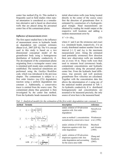Together with the concentration data this allows the determination of � using any of the analytical models presented in Tab. 1. As hydraulic conductivity K is distributed homogeneously and concentrations are assumed to be measured precisely, the only source of error here is the measured head. Tab. 1: Analytical models for the estimation of the first order degradation rate constant �. method formula description reference 1 2 3 4 v � � a C ( x) � � � � � � � 1 ln �x � C0 � v � � � a � C ( x) C0 � � � � 2 ln �x � C � � � 0 C ( x) � with �C( x) C � 2 v � � a �� ln 0 � � � � 3 � � �1 � 2� L � 1 4� � L �� x � � �C( x) ( C � ) � 2 v � � a �� ln 0 � � � � 4 � � �1 � 2� L � 1 4� � L �� x � � � � � W S � � erf � � � � 4 � T � x � analyt. solution of 1D advection equation with first order degradation same as method 1; concentrations normalized by conservative tracer analyt. solution of 1D advectiondispersion equation with first order degradation analyt. solution of 2D advectiondispersion equation with first order degradation and accounting for the source area width . Newell et al. (2002) Wiedemeyer et al. (1996) Buscheck and Alcantar (1995) Zhang and Heathcote (2003) 11
Page 3 and 4: Applied numerical modeling of satur
Page 5: Abstract Applied numerical modeling
Page 9: Vorwort Die zurückliegenden drei J
Page 13: List of abbreviations and mathemati
Page 16 and 17: for the application studies outline
Page 18 and 19: path lengths of water molecules tha
Page 20 and 21: where vmax [s -1 ] is a maximum gro
Page 22 and 23: domain is discretized along advecti
Page 26 and 27: The conceptual model used is a rigo
Page 28 and 29: equires therefore a higher degradat
Page 30 and 31: studied for heterogeneous sites wit
Page 32 and 33: Fig. 13: Plume length overestimatio
Page 34 and 35: concentration maximum is for the ca
Page 36 and 37: possibilities can not be provided n
Page 38 and 39: technischen Bauwerken. (Model based
Page 40 and 41: Schäfer, D., Dahmke, A., Kolditz,
Page 43: Enclosed Publication 1 Bauer, S., B
Page 46 and 47: Assessing measurements of first-ord
Page 55 and 56: WATER RESOURCES RESEARCH, VOL. 42,
Page 57 and 58: W01420 BAUER ET AL.: ASSESSING FIRS
Page 69: Enclosed Publication 3 Beyer, C., B
Page 72 and 73: 74 C. Beyer et al. / Journal of Con
Page 74 and 75:
76 C. Beyer et al. / Journal of Con
Page 76 and 77:
Page 78 and 79:
Page 80 and 81:
Page 82 and 83:
Page 84 and 85:
Page 86 and 87:
Page 88 and 89:
Page 90 and 91:
Page 92 and 93:
Page 95:
Enclosed Publication 4 Bauer, S., B
Page 98 and 99:
Einführung In dieser Arbeit wird e
Page 100 and 101:
Entlang der so bestimmten Grundwass
Page 102 and 103:
Für die letztgenannten Methoden m
Page 104 and 105:
Um diesen Effekt zu verdeutlichen s
Page 106 and 107:
Unsicherheit zu. Für Methode 3 ( A
Page 108 and 109:
sagt sowie die zusätzliche Problem
Page 111:
Enclosed Publication 5 Beyer, C., C
Page 114 and 115:
(1995) yields a “hybrid” rate c
Page 116 and 117:
2 integral scale lY of 2.67 m and l
Page 118 and 119:
The approximate solution employed h
Page 120 and 121:
As Bauer et al. (2006a) demonstrate
Page 122 and 123:
Table 4: Normalized degradation rat
Page 124 and 125:
Comparing results for source widths
Page 127:
Enclosed Publication 6 Beyer, C., K
Page 130 and 131:
Einleitung und Zielsetzung In Deuts
Page 132 and 133:
die Anzahl Simulationsläufe den Vo
Page 134 and 135:
Grundlage des Korngrößenspektrums
Page 136 and 137:
Dies ist als konservative Abschätz
Page 138 and 139:
Randbedingungen abhängig ist. Aus
Page 140 and 141:
keinen Einfluss auf die abgebaute M
Page 142 and 143:
Carsell, R. F., Parish, R. S.: Deve
Page 144:
van Genuchten, M.T.: A closed form
show all

Applied numerical modeling of saturated / unsaturated flow and ...

You also want an ePaper? Increase the reach of your titles

Delete template?

Save as template?