Low (web) Quality - BALTEX

232
Regional climate simulation with mosaic GCMs
Michel Déqué
Météo-France/CNRM, CNRS/GAME, 42 avenue Coriolis, 31057 Toulouse Cédex 1, France; deque@meteo.fr
1. Introduction
The next IPCC exercise will include contributions of
regional models on areas of the globe that have not be
covered in the past by international multimodel projects
like NARCCAP or ENSEMBLES. The target resolution
will be 50 km. Ideally, the best exercise would be to run a
global model at 50 km resolution driven by sea surface
temperatures (SST) from lower resolution coupled model.
If local biases in SST are too detrimental to some
regional climates, they can be corrected. But such an
exercise is unaffordable for many modelling groups, and
very heavy (e.g. ARPEGE model needs one year with a
full 8-processor node on a NEC-SX8 computer) for other
groups. A more flexible approach is proposed here.
2. Scope of the study
The ARPEGE model has the capability of variable
resolution with maximum resolution around a pole of
interest. If the whole globe is considered, then several
poles must be used, and then several versions of the
model must be run. Given well known geometrical
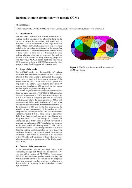
properties of the sphere, a good number of poles is 20,
because the icosahedron (20 vertices) is the largest
possible regular polyhedron (see Figure 1).
Two AMIP 10-year experiments are used for the analysis.
They use each versions of ARPEGE at different poles.
The spectral truncation is TL179 and the stretching factor
is two. If we build a composite grid with the maximum
resolution everywhere, the mean resolution is 57 km with
a maximum of 54 km and a minimum of 65 km. If we
consider an individual model, the minimum resolution (at
the antipodes) is 200 km. In the first experiment, the
models are run independently. It is possible to build
composites of climate parameters like seasonal mean or
standard deviation. But it is not possible to reconstruct
daily fields, because each run has its own history, and
using the same SST is not enough to constrain the
atmosphere daily fields. Thus a second experiment is
proposed. A preliminary AMIP simulation has been run
by the same model with homogeneous TL159 120 km
horizontal resolution. This is the “pacemaker” simulation.
Then the variable resolution models are run with driving
conditions from this run. For each model, the relaxation
coefficient is zero where the resolution is the maximum
of the 20 grids, and maximum (6-hour e-folding time)
where the resolution is less than that of the driving model
(i.e. 120 km).
Figure 1: The 20 equal-area on which a stretched
GCM may focus.
3. Content of the presentation
In the presentation, we will use eight such GCMs
surrounding Europe and Africa. The reference is a 10-
year run with a version of ARPEGE at homogeneous
TL319 60 km resolution (perfect model exercise). We
will analyze the effects of the “seams” in the composite
fields and examine whether imposing a relaxation is
detrimental to or improving the simulation in the area of
high resolution.