Low (web) Quality - BALTEX
Low (web) Quality - BALTEX
Low (web) Quality - BALTEX

Create successful ePaper yourself
Turn your PDF publications into a flip-book with our unique Google optimized e-Paper software.
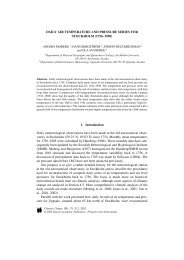
32<br />
The geographical distribution of interannual variability of<br />
500 hPa height in summer, shown in Figure 2 (first row),<br />
clearly demonstrates where the error dominates. The<br />
variability is nearly the same between R-2 and the new<br />
version of SSBC, while the run without SSBC significantly<br />
increase the interannual variability in the area near the center<br />
of the domain, where the variability is more than 30% larger<br />
than R-2. During the winter (Fig. 2, second row), the<br />
patterns of interannual variability between R2 and NOSSBA<br />
are not far apart, although without SSBC, the variability is<br />
enhanced by 10-20% in the middle of the region. The<br />
difference in interannual variability becomes more apparent<br />
when the variability is decomposed into EOFs (Figure 3).<br />
The first mode (top row) in no SSBC (second column) has<br />
quite different pattern than the others. Apparently, the<br />
regional model error produces its own interannual variability<br />
and contaminates the low frequency variability in the global<br />
forcing. Mode 2 (2 nd row) for no SSBC (second column) is<br />
also very different from R2 and others. The original SSBC<br />
corrects most of the error in EOFs, but the refined SSBC<br />
makes the EOF patterns much closer to those of the R-2.<br />
Mode 1<br />
Mode 2<br />
R2<br />
NOSSBC<br />
SSBC<br />
32% 38%<br />
32%<br />
32%<br />
19% 20% 15% 18%<br />
NEWSSB<br />
C<br />
Figure 3. Leading two modes of summer time 500<br />
hPa geopotential height EOF for analysis (R2) and<br />
experiments during summer. The percent variance is<br />
indicated by percent in each panel.<br />
The linear trend is also affected by the model error, which is<br />
shown in Figure 4. The patterns and magnitudes of the<br />
linear trends are very different when no correction is<br />
applied, while correction works well to correct the problem.<br />
summer winter<br />
R-2<br />
NOSSBC<br />
SSBC<br />
NEWSSBC<br />
Figure 4. 1972-2005 linear trend of 500 hPa height<br />
for summer (upper panels) and winter (lower panels).<br />
Unit in meter/10 years.<br />
Figure 5 is the EOF of precipitation during summer for<br />
Mode 1, the patterns of model simulations are not so close to<br />
the observed pattern, but NEWSSBC and SSBC resemble<br />
more with CMAP than that of NOSSBC. Somewhat<br />
disorganized EOF patterns in model simulations indicate<br />
that the model response is weaker to interannual variability<br />
in large scale forcing, but the correction of large scale<br />
certainly helps in improving the simulation of precipitation<br />
variability.<br />
Mode<br />
1<br />
Mode<br />
2<br />
4. Conclusions<br />
In this paper, it is demonstrated that conventional<br />
dynamical downscaling methods without any large scale<br />
error corrections suffer from large scale regional model<br />
error that contaminates interannual variability and linear<br />
trend of downscaled fields. The error also contaminates<br />
low frequency variability and trend of derived fields, such<br />
as precipitation. The effect of model error on the<br />
variability is greater in summer time, as the magnitude of<br />
the error is comparable to the interannual variability of<br />
seasonal mean.<br />
CMAP<br />
NOSSBC<br />
SSBC<br />
NEWSSBC<br />
27% 17% 17% 23%<br />
15% 10% 9% 15%<br />
Figure 5. First two leading EOF of seasonal mean<br />
precipitation during summer from observation (R-2) and<br />
experiments.<br />
These errors can be corrected nicely by introducing Scale<br />
Selective Bias Correction method. However, the impact<br />
of correcting large scale error in simulating precipitation<br />
and near surface temperature was found to be modest.<br />
This somewhat reduced impact is due to the inaccuracies<br />
in the precipitation process in the model, which is not able<br />
to faithfully reproduce observed precipitation given large<br />
scale forcing, particularly its interannual variability.<br />
However, the modest impact implies that even with<br />
somewhat deficient parameterization, the correction to<br />
large scale forcing works positively to reduce error and<br />
improve dynamical downscaling.<br />
The large scale model error examined in this paper would<br />
be a strong function of the choice of the model domain, its<br />
location, model resolution and physics of the model. It is<br />
very likely that the error increases as the domain size<br />
increase. In this regard, it seems important to apply<br />
SSBC to all the cases, which have a potential of improving<br />
the simulations of mean as well as interannual variability.<br />
Regarding the use of SSBC in the downscaling of GCM<br />
simulations, for which truth is not known, our<br />
recommendation is to utilize it fully. Although it is not<br />
possible to obtain large scale regional model error, it is<br />
more logical to faithfully apply the large scale forcing<br />
simulated by the global model without altering it by the<br />
regional model. It should be emphasized again that the<br />
dynamical downscaling is a diagnostic tool to obtain small<br />
scale features forced by given large scale forcing, thus the<br />
large scale forcing should not be modified during the<br />
downscaling procedure.<br />
References<br />
Alexandru, A., R. de Elia, and R. Laprise, 2007: Internal<br />
variability in regional climate downscaling at the<br />
seasonal scale Mon. Wea. Rev. 135, 3221–3238<br />
Kanamaru H. and M. Kanamitsu, 2006: Scale selective<br />
bias correction in a downscaling of global analysis<br />
using a regional model, Mon. Wea. Rev.135, 334-350.<br />
Kanamitsu, M. and H. Kanamaru, 2007: 57-year<br />
California Reanalysis downscaling at 10km (CaRD10)<br />
Part I. System detail and validation with observations.<br />
J. Climate, 20, 5527-5552.