1 Montgomery Modular Multiplication in Hard- ware

FEI KEMT
embedded processor with a set of dedicated coprocessors. For such a system a
highly flexible (although typically slower) scalable MMM coprocessor could be more
attractive than a fixed length dedicated one.
That direction was chosen in our research, when our goal is to analyse and
implement solution that would allow quick prototyping of special purpose hardware
designs and use features of target platform in order to accelerate execution of the
MMM operation.
The radix-2 MMM algorithm (b = 2) is very suitable for hardware implemen-
tation due to easily implementable operations as a word-by-bit multiplication, a
bit-shift (division by two) and an addition. Implementations with higher radix were
also published [30, 110] and offer a proper alternative, but using a more complex
algebraic unit.
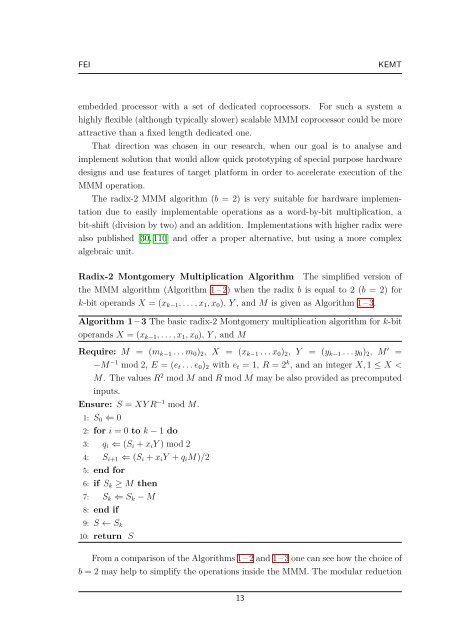
Radix-2 Montgomery Multiplication Algorithm The simplified version of
the MMM algorithm (Algorithm 1 – 2) when the radix b is equal to 2 (b = 2) for
k-bit operands X = (xk−1, . . . , x1, x0), Y , and M is given as Algorithm 1 – 3.
Algorithm 1 – 3 The basic radix-2 Montgomery multiplication algorithm for k-bit
operands X = (xk−1, . . . , x1, x0), Y , and M
Require: M = (mk−1 . . . m0)2, X = (xk−1 . . . x0)2, Y = (yk−1 . . . y0)2, M ′ =
−M −1 mod 2, E = (et . . . e0)2 with et = 1, R = 2 k , and an integer X, 1 ≤ X <
M. The values R 2 mod M and R mod M may be also provided as precomputed
inputs.
Ensure: S = XY R −1 mod M.
1: S0 ⇐ 0
2: for i = 0 to k − 1 do
3: qi ⇐ (Si + xiY ) mod 2
4: Si+1 ⇐ (Si + xiY + qiM)/2
5: end for
6: if Sk ≥ M then
7: Sk ⇐ Sk − M
8: end if
9: S ← Sk
10: return S
From a comparison of the Algorithms 1 – 2 and 1 – 3 one can see how the choice of
b = 2 may help to simplify the operations inside the MMM. The modular reduction
13