Méthodes de Monte Carlo appliquées au pricing d ... - Maths-fi.com

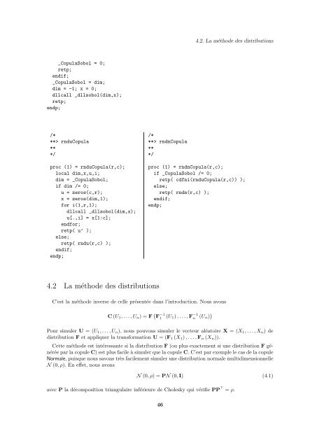
4.2. La méthode des distributions_CopulaSobol = 0;retp;endif;_CopulaSobol = dim;dim = -1; x = 0;dllcall _dllsobol(dim,x);retp;endp;/***> rnduCopula***/proc (1) = rnduCopula(r,c);local dim,x,u,i;dim = _CopulaSobol;if dim /= 0;u = zeros(c,r);x = zeros(dim,1);for i(1,r,1);dllcall _dllsobol(dim,x);u[.,i] = x[1:c];endfor;retp( u’ );else;retp( rndu(r,c) );endif;endp;/***> rndnCopula***/proc (1) = rndnCopula(r,c);if _CopulaSobol /= 0;retp( cdfni(rnduCopula(r,c)) );else;retp( rndn(r,c) );endif;endp;4.2 La méthode des distributionsC’est la méthode inverse de celle présentée dans l’introduction. Nous avonsC (U 1 , . . . , U n ) = F ( F −11 (U 1 ) , . . . , F −1n (U n ) )Pour simuler U = (U 1 , . . . , U n ), nous pouvons simuler le vecteur aléatoire X = (X 1 , . . . , X n ) dedistribution F et appliquer la transformation U = (F 1 (X 1 ) , . . . , F n (X n )).Cette méthode est intéressante si la distribution F (ou plus exactement si une distribution F généréepar la copule C) est plus facile à simuler que la copule C. C’est par exemple le cas de la copuleNormale, puisque nous savons très facilement simuler une distribution normale multidimensionnelleN (0, ρ). En effet, nous avonsN (0, ρ) = PN (0, I) (4.1)avec P la décomposition triangulaire inférieure de Cholesky qui vérifie PP ⊤ = ρ.46