MÃ©thodes de Monte Carlo appliquÃ©es au pricing d ... - Maths-fi.com

More documents

Recommendations

Info

4.2. La méthode des distributions_CopulaSobol = 0;retp;endif;_CopulaSobol = dim;dim = -1; x = 0;dllcall _dllsobol(dim,x);retp;endp;/***> rnduCopula***/proc (1) = rnduCopula(r,c);local dim,x,u,i;dim = _CopulaSobol;if dim /= 0;u = zeros(c,r);x = zeros(dim,1);for i(1,r,1);dllcall _dllsobol(dim,x);u[.,i] = x[1:c];endfor;retp( u’ );else;retp( rndu(r,c) );endif;endp;/***> rndnCopula***/proc (1) = rndnCopula(r,c);if _CopulaSobol /= 0;retp( cdfni(rnduCopula(r,c)) );else;retp( rndn(r,c) );endif;endp;4.2 La méthode des distributionsC’est la méthode inverse de celle présentée dans l’introduction. Nous avonsC (U 1 , . . . , U n ) = F ( F −11 (U 1 ) , . . . , F −1n (U n ) )Pour simuler U = (U 1 , . . . , U n ), nous pouvons simuler le vecteur aléatoire X = (X 1 , . . . , X n ) dedistribution F et appliquer la transformation U = (F 1 (X 1 ) , . . . , F n (X n )).Cette méthode est intéressante si la distribution F (ou plus exactement si une distribution F généréepar la copule C) est plus facile à simuler que la copule C. C’est par exemple le cas de la copuleNormale, puisque nous savons très facilement simuler une distribution normale multidimensionnelleN (0, ρ). En effet, nous avonsN (0, ρ) = PN (0, I) (4.1)avec P la décomposition triangulaire inférieure de Cholesky qui vérifie PP ⊤ = ρ.46
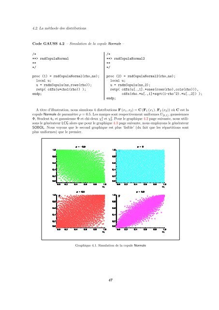
4.2. La méthode des distributionsCode GAUSS 4.2 – Simulation de la copule Normale –/***> rndCopulaNormal***/proc (1) = rndCopulaNormal(rho,ns);local u;u = rndnCopula(ns,rows(rho));retp( cdfn(u*chol(rho)) );endp;/***> rndCopulaNormal2***/proc (2) = rndCopulaNormal2(rho,ns);local u;u = rndnCopula(ns,2);retp( cdfn(u[.,1].*ones(rows(rho),cols(rho))),cdfn(rho.*u[.,1]+sqrt(1-rho^2).*u[.,2]) );endp;A titre d’illustration, nous simulons 4 distributions F (x 1 , x 2 ) = C (F 1 (x 1 ) , F 2 (x 2 )) où C est lacopule Normale de paramètre ρ = 0.5. Les marges sont respectivement uniformes U [0,1] , gaussiennesΦ, Student t 5 et gaussienne Φ et chi-deux χ 2 1 et χ 2 8. Pour le graphique 4.2 page suivante, nous utilisonsle générateur LCG alors que pour le graphique 4.3 page suivante, nous employons le générateurSOBOL. Nous voyons que le second graphique est plus ‘lisible’ (du fait que les répartitions sontplus uniformes) que le premier.Graphique 4.1. Simulation de la copule Normale47
Page 3: Table des matières1 Simulation d
Page 6 and 7: 1.1. Générateurs congruentiels li
Page 8 and 9: 1.2. Tests d’uniformitéqu’en d
Page 10 and 11: 1.2. Tests d’uniformitéCes valeu
Page 12: 1.3. Autres types de générateursL
Page 15 and 16: 2Simulation d’une loi non uniform
Page 17 and 18: 2.2. Méthode des transformations2.
Page 19 and 20: 2.2. Méthode des transformationsmi
Page 21 and 22: 2.3. Le cas des distributions discr
Page 23 and 24: 2.3. Le cas des distributions discr
Page 25 and 26: 2.4. La méthode des mélanges disc
Page 27 and 28: 2.5. Simulation par acceptation-rej
Page 33 and 34: 3Méthodes de Monte Carlo appliqué
Page 35 and 36: 3.2. Variables de contrôleSi v g c
Page 37 and 38: 3.2. Variables de contrôleSi l’o
Page 39 and 40: 3.3. Échantillonnage d’importanc
Page 47 and 48: 3.4. Stratificationil peut être in
Page 49: 4Utilisation des copules pour la si
Page 53 and 54: 4.2. La méthode des distributionsC
Page 55 and 56: 4.3. La méthode des distributions
Page 61 and 62: 4.5. La méthode des quantiles empi
Page 63 and 64: 5Méthodes de Monte Carlo appliqué
Page 65 and 66: 5.1. Le problème de l’agrégatio
Page 67 and 68: 5.2. Différentes méthodes de cons
Page 75 and 76: 5.3. Calcul de la charge en capital
Page 81 and 82: Bibliographie[1] Bouyé, E., V. Dur

MÃ©thodes de Monte Carlo appliquÃ©es au pricing d ... - Maths-fi.com

You also want an ePaper? Increase the reach of your titles

Delete template?

Save as template?