Segmentation of Stochastic Images using ... - Jacobs University

Chapter 7 Stochastic Level Sets
MC SC PC
E
Var
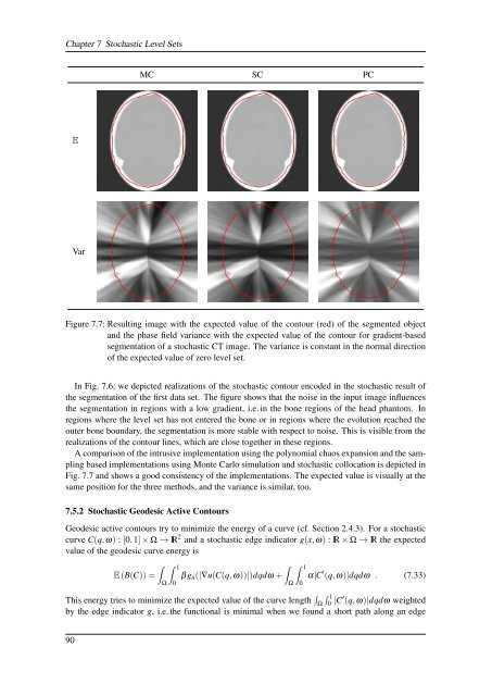
Figure 7.7: Resulting image with the expected value of the contour (red) of the segmented object
and the phase field variance with the expected value of the contour for gradient-based
segmentation of a stochastic CT image. The variance is constant in the normal direction
of the expected value of zero level set.
In Fig. 7.6, we depicted realizations of the stochastic contour encoded in the stochastic result of
the segmentation of the first data set. The figure shows that the noise in the input image influences
the segmentation in regions with a low gradient, i.e. in the bone regions of the head phantom. In
regions where the level set has not entered the bone or in regions where the evolution reached the
outer bone boundary, the segmentation is more stable with respect to noise. This is visible from the
realizations of the contour lines, which are close together in these regions.
A comparison of the intrusive implementation using the polynomial chaos expansion and the sampling
based implementations using Monte Carlo simulation and stochastic collocation is depicted in
Fig. 7.7 and shows a good consistency of the implementations. The expected value is visually at the
same position for the three methods, and the variance is similar, too.
7.5.2 Stochastic Geodesic Active Contours
Geodesic active contours try to minimize the energy of a curve (cf. Section 2.4.3). For a stochastic
curve C(q,ω) : [0,1] × Ω → IR 2 and a stochastic edge indicator g(x,ω) : IR × Ω → IR the expected
value of the geodesic curve energy is
∫ ∫ 1
∫ ∫ 1
E(B(C)) = βg u (|∇u(C(q,ω))|)dqdω + α|C ′ (q,ω)|dqdω . (7.33)
Ω 0
Ω 0
This energy tries to minimize the expected value of the curve length ∫ Ω
∫ 1
0 |C′ (q,ω)|dqdω weighted
by the edge indicator g, i.e. the functional is minimal when we found a short path along an edge
90