Segmentation of Stochastic Images using ... - Jacobs University

Chapter 7 Stochastic Level Sets
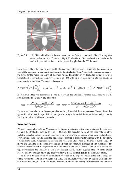
Figure 7.11: Left: MC-realizations of the stochastic contour from the stochastic Chan-Vese segmentation
applied on the CT data set. Right: Realizations of the stochastic contour from the
stochastic geodesic active contour approach applied on the CT data set.
noise levels. Thus, they can be separated by homogenizing the variance. To include the homogenization
of the variance we add additional terms to the stochastic Chan-Vese model that are inspired by
the terms for the homogenization of the mean value. The inclusion of stochastic moments in functionals
has been investigated e.g. by Tiesler et al. [146]. To be more precise, we add two additional
components to the Chan-Vese energy leading to
( ( )
∇φ
φ t = δ ε (φ) µ∇·
)−ν −λ 1 (u 0 − c 1 ) 2 +λ 2 (u 0 − c 2 ) 2 −ρ 1 (Var(u 0 ) − v 1 ) 2 +ρ 2 (Var(u 0 )−v 2 ) 2 .
|∇φ|
(7.41)
In (7.41) we added two parameters ρ 1 and ρ 2 to weight the additional components. Furthermore, the
new components v 1 and v 2 are defined as
∫
D
v 1 (φ) =
Var(u 0(x))H ε (φ(x))dx
∫
D H ε(φ(x))dx
∫
and v 2 (φ) =
D Var(u 0(x))(1 − H ε (φ(x)))dx
∫
D (1 − H ε(φ(x)))dx
. (7.42)
Remember, the variance can be computed from the polynomial chaos expansion of the stochastic image
easily. Moreover, it is possible to homogenize every polynomial chaos coefficient independently,
leading to various additional constraints.
Numerical Results
We apply the stochastic Chan-Vese model on the same data sets as the other methods: the stochastic
CT and the stochastic liver mask. Fig. 7.10 shows the expected value of the liver data set along
with the expected value contour at stages of the evolution. The stochastic Chan-Vese model slightly
overestimates the object, because the final (green) contour is not perfectly aligned with the boundary.
This is due to the homogenization criterion the stochastic Chan-Vese model tries to fulfill. Fig. 7.10
shows the variance of the final level set along with the contours at stages of the evolution. The
variance indicated that the segmentation is uncertain in the critical areas at the object’s bottom and
top. Furthermore, the variance identifies two critical regions on the right and the left of the object.
Fig. 7.11 shows realizations of the final contour via a MC-sampling from the stochastic result.
For the liver data set, we show the level set evolution on the expected value of the initial image and
on the variance of the final level set in Fig. 7.12. The data set is constructed by adding artificial noise
to a noise-free image. This noise nearly cancels out due to the averaging process for the computa-
94