Segmentation of Stochastic Images using ... - Jacobs University

More documents

Recommendations

Info

Chapter 6 Segmentation of Stochastic Images Using Elliptic SPDEs Figure 6.10: Nonzero pattern of the SFEM matrix for the smoothed stochastic image using n = 5 random variables and a polynomial degree p = 3. A black dot denotes a block that has a nonzero stochastic part, thus having the sparsity structure of a classical FEM matrix. for all β ∈ {1,...,N}, where M α,β ,L α,β ,S α,β and T α,β are blocks of the system matrix, defined as (M α,β ) i, j = E (Ψ α Ψ β ) ∫ (S α,β ) i, j = E (Ψ α Ψ β ) ∫ D D P i P j dx , ∇P i · ∇P j dx (6.26) and ( ( L α,β ) i, j = ∑ k T α,β ) i, j = ∑ k ( ∑E Ψ α Ψ β Ψ γ) ∫ (˜φ 2 ) k γ γ ∫ ∑E γ ( Ψ α Ψ β Ψ γ) u k γ D D ∇P i · ∇P j P k dx , P i P j P k dx . (6.27) Here, (˜φ 2 ) k γ denotes a coefficient of the polynomial chaos expansion of the Galerkin projection of φ 2 onto the image space (cf. Section 3.3.3). The right hand side vector of the phase field equation is ∫ (A α ) i = Γ ∫ Ψ α dΠ D ⎧ ∫ 1 ⎪⎨ 4ε P i dx = D ⎪⎩ 1 4ε P i dx if α = 1 , 0 else . (6.28) Note that the expectations of the products of stochastic basis functions involved above are again the components of the lookup table introduced in Section 3.3.5. The deterministic integrals can be precomputed, because they are needed several times during the assembling of the system matrix. Analog to the classical finite element method the systems of linear equations can be treated by an iterative solver like the method of conjugate gradients [67]. The general block structure of an SFEM matrix is depicted in Fig. 6.9 and the sparsity structure on the block level for five random variables and a polynomial degree of three is depicted in Fig. 6.10. In addition, the matrix generation can be accelerated using lookup tables. The memory consumption is enormous, because the matrix has N 2 -times the storage requirement of the deterministic matrix, where N is the dimension of the polynomial chaos. Thus, we use the GSD method for the solution to avoid the generation of the SFEM matrix. 70
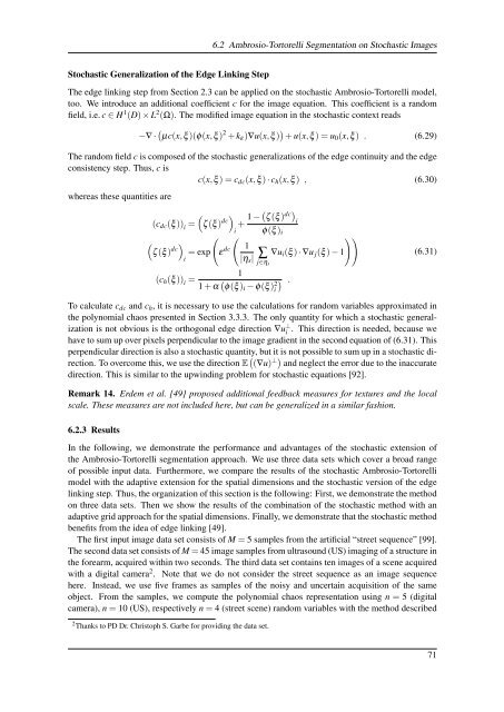
6.2 Ambrosio-Tortorelli Segmentation on Stochastic Images Stochastic Generalization of the Edge Linking Step The edge linking step from Section 2.3 can be applied on the stochastic Ambrosio-Tortorelli model, too. We introduce an additional coefficient c for the image equation. This coefficient is a random field, i.e. c ∈ H 1 (D) × L 2 (Ω). The modified image equation in the stochastic context reads −∇ · (µc(x,ξ )(φ(x,ξ ) 2 + k ε )∇u(x,ξ ) ) + u(x,ξ ) = u 0 (x,ξ ) . (6.29) The random field c is composed of the stochastic generalizations of the edge continuity and the edge consistency step. Thus, c is c(x,ξ ) = c dc (x,ξ ) · c h (x,ξ ) , (6.30) whereas these quantities are ( (c dc (ξ )) i = ζ (ξ ) dc) + 1 − ( ζ (ξ ) dc) i i φ(ξ ) i ( ( )) ( ζ (ξ ) dc) = exp ε dc 1 i |η s | ∑ ∇u i (ξ ) · ∇u j (ξ ) − 1 j∈η s 1 (c h (ξ )) i = 1 + α ( ) φ(ξ ) i − φ(ξ ) 2 . i (6.31) To calculate c dc and c h , it is necessary to use the calculations for random variables approximated in the polynomial chaos presented in Section 3.3.3. The only quantity for which a stochastic generalization is not obvious is the orthogonal edge direction ∇u ⊥ i . This direction is needed, because we have to sum up over pixels perpendicular to the image gradient in the second equation of (6.31). This perpendicular direction is also a stochastic quantity, but it is not possible to sum up in a stochastic direction. To overcome this, we use the direction E ( (∇u) ⊥) and neglect the error due to the inaccurate direction. This is similar to the upwinding problem for stochastic equations [92]. Remark 14. Erdem et al. [49] proposed additional feedback measures for textures and the local scale. These measures are not included here, but can be generalized in a similar fashion. 6.2.3 Results In the following, we demonstrate the performance and advantages of the stochastic extension of the Ambrosio-Tortorelli segmentation approach. We use three data sets which cover a broad range of possible input data. Furthermore, we compare the results of the stochastic Ambrosio-Tortorelli model with the adaptive extension for the spatial dimensions and the stochastic version of the edge linking step. Thus, the organization of this section is the following: First, we demonstrate the method on three data sets. Then we show the results of the combination of the stochastic method with an adaptive grid approach for the spatial dimensions. Finally, we demonstrate that the stochastic method benefits from the idea of edge linking [49]. The first input image data set consists of M = 5 samples from the artificial “street sequence” [99]. The second data set consists of M = 45 image samples from ultrasound (US) imaging of a structure in the forearm, acquired within two seconds. The third data set contains ten images of a scene acquired with a digital camera 2 . Note that we do not consider the street sequence as an image sequence here. Instead, we use five frames as samples of the noisy and uncertain acquisition of the same object. From the samples, we compute the polynomial chaos representation using n = 5 (digital camera), n = 10 (US), respectively n = 4 (street scene) random variables with the method described 2 Thanks to PD Dr. Christoph S. Garbe for providing the data set. 71
Page 1:
Segmentation of Stochastic Images u
Page 5:
Abstract The task of segmentation,
Page 8 and 9:
7.5 Segmentation of Stochastic Imag
Page 11 and 12:
Chapter 1 Introduction The developm
Page 13 and 14:
Figure 1.3: This thesis combines fi
Page 15:
the presentation of the stochastic
Page 18 and 19:
Chapter 2 Image Segmentation and Li
Page 20 and 21:
Page 22 and 23:
Page 24 and 25:
Page 26 and 27:
Page 28 and 29:
Page 30 and 31: Chapter 2 Image Segmentation and Li
Page 36 and 37: Chapter 3 SPDEs and Polynomial Chao
Page 48 and 49: Chapter 4 Discretization of SPDEs F
Page 50 and 51: Chapter 4 Discretization of SPDEs 4
Page 52 and 53: Chapter 4 Discretization of SPDEs a
Page 58 and 59: Chapter 5 Stochastic Images
Page 60 and 61: Chapter 5 Stochastic Images Figure
Page 62 and 63: Chapter 5 Stochastic Images like qu
Page 64 and 65: Chapter 5 Stochastic Images Figure
Page 67 and 68: Chapter 6 Segmentation of Stochasti
Page 69 and 70: 6.1 Random Walker Segmentation on S
Page 77 and 78: 6.2 Ambrosio-Tortorelli Segmentatio
Page 79: 6.2 Ambrosio-Tortorelli Segmentatio
Page 87: 6.2 Ambrosio-Tortorelli Segmentatio
Page 90 and 91: Chapter 7 Stochastic Level Sets whe
Page 92 and 93: Chapter 7 Stochastic Level Sets Fig
Page 94 and 95: Chapter 7 Stochastic Level Sets and
Page 96 and 97: Chapter 7 Stochastic Level Sets rar
Page 100 and 101: Chapter 7 Stochastic Level Sets MC
Page 106 and 107: Chapter 7 Stochastic Level Sets act
Page 108 and 109: Chapter 8 Segmentation of Classical
Page 118 and 119: Chapter 9 Summary, Discussion, and
Page 121 and 122: List of Figures 1.1 Left: CT image
Page 123 and 124: List of Figures 6.2 Mean and varian
Page 125: List of Figures 7.12 Mean (left) of
Page 129 and 130: Appendix A Publications Written Dur
Page 131 and 132:
Bibliography [14] L. Ambrosio and M
Page 133 and 134:
Bibliography [46] B. Echebarria, R.
Page 135 and 136:
Bibliography [81] B. N. Khoromskij
Page 137 and 138:
Bibliography [113] A. Nouy. A gener
Page 139:
Bibliography [147] J. Tryoen, O. Le
show all

Segmentation of Stochastic Images using ... - Jacobs University

Create successful ePaper yourself

Delete template?

Save as template?