Segmentation of Stochastic Images using ... - Jacobs University

6.2 Ambrosio-Tortorelli Segmentation on Stochastic Images
✛
✛
j
✻
i
❄
✲
α
✲
✻ + L α,β
✟ ✟✟✟✟✟Mα,β β
❄
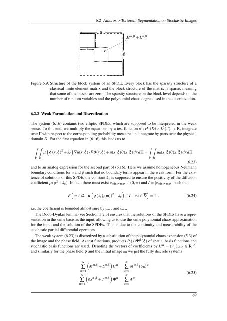
Figure 6.9: Structure of the block system of an SPDE. Every block has the sparsity structure of a
classical finite element matrix and the block structure of the matrix is sparse, meaning
that some of the blocks are zero. The sparsity structure on the block level depends on the
number of random variables and the polynomial chaos degree used in the discretization.
6.2.2 Weak Formulation and Discretization
The system (6.16) contains two elliptic SPDEs, which are supposed to be interpreted in the weak
sense. To this end, we multiply the equations by a test function θ : H 1 (D) × L 2 (Γ) → IR, integrate
over Γ with respect to the corresponding probability measure, and integrate by parts over the physical
domain D. For the first equation in (6.16) this leads us to
∫
Γ
∫
D
)
∫
µ
(φ (x,ξ ) 2 + k ε ∇u(x,ξ ) · ∇θ(x,ξ ) + u(x,ξ )θ(x,ξ )dxdΠ =
Γ
∫
D
u 0 (x,ξ )θ(x,ξ )dxdΠ
(6.23)
and to an analog expression for the second part of (6.16). Here we assume homogeneous Neumann
boundary conditions for u and φ such that no boundary terms appear in the weak form. For the existence
of solutions of this SPDE, the constant k ε is supposed to ensure the positivity of the diffusion
coefficient µ(φ 2 + k ε ). In fact, there must exist c min ,c max ∈ (0,∞) and I = [c min ,c max ] such that
(
P ω ∈ Ω ∣ )
µ
(φ (x,ξ (ω)) 2 + k ε ∈ I
)
∀x ∈ D = 1 , (6.24)
i.e. the coefficient is bounded almost sure by c min and c max .
The Doob-Dynkin lemma (see Section 3.2.3) ensures that the solutions of the SPDEs have a representation
in the same basis as the input, allowing us to use the same polynomial chaos approximation
for the input and the solution of the SPDEs. This is due to the continuity and measurability of the
stochastic partial differential operators.
The weak system (6.23) is discretized by a substitution of the polynomial chaos expansion (5.3) of
the image and the phase field. As test functions, products P j (x)Ψ β (ξ ) of spatial basis functions and
stochastic basis functions are used. Denoting the vectors of coefficients by U α = (u i α) i∈I ∈ IR |I |
and similarly for the phase field φ and the initial image u 0 we get the fully discrete systems
N (
∑
) M α,β + L α,β U α =
α=1
(
N
∑
α=1
εS α,β + T α,β ) Φ α =
N
∑
α=1
N
∑
α=1
M α,β (U 0 ) α
A α (6.25)
69