Segmentation of Stochastic Images using ... - Jacobs University

Chapter 5 Stochastic Images
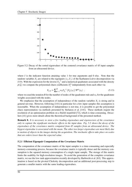
Figure 5.2: Decay of the sorted eigenvalues of the centered covariance matrix of 45 input samples
from an ultrasound device.
where I is the indicator function attaining value 1 for true arguments and 0 else. Note that the
random variables X j are related to the eigenpairs (s j ,U j ) of the Karhunen-Loève decomposition via
(5.9). With the expression for the inverse FX −1
j
and a numerical quadrature associated with the density
ρ(ξ ) we compute the polynomial chaos coefficients Xj
α independently from each other via
X j,α ≈ ∑ R k=1 w kF −1
X j
(
Fξ (y k ) ) Ψ α (y k ) , (5.13)
where we used the notation R for the number of nodes of the quadrature rule and w k for the quadrature
weights associated with the nodes.
We emphasize that the assumption of independence of the random variables X j is strong and in
general not true. However, following [141] in particular for a few input samples this assumption is
reasonable. When the assumption of independence is not true, it is possible to get the polynomial
chaos representation via methods presented by Stefanou et al. [141]. These methods require the
resolution of an optimization problem on a Stiefel manifold [72], which is time-consuming. Desceliers
[41] gives more details about the theoretical background of the presented method.
Remark 8. It is necessary to store a few leading eigenvalues and eigenvectors of the covariance
only to capture the significant stochastic effects in the input data. Fig. 5.2 shows the decay of the
eigenvalues of the covariance matrix computed from 45 samples from an ultrasound device. The
biggest eigenvalue is associated with the mean. The other two larger eigenvalues are most likely due
to motion of objects in the images during the acquisition. The stochastic effects take place on scales
that are orders lower than the expected value.
5.2.1 Efficient Eigenpair Computation of the Covariance Matrix
The computation of the covariance matrix of the input samples is a time-consuming and especially
memory-consuming process, because the covariance matrix is typically dense and the memory consumption
is the squared memory consumption of a single input sample. The storage of this matrix
limits the usability for high-resolution images. To avoid the generation of the complete covariance
matrix, we use the low rank approximation recently developed by Harbrecht et al. [63]. This approximation
is based on the pivoted Cholesky decomposition and an additional post-processing step to
generate a smaller matrix with the same leading eigenvalues.
50