Segmentation of Stochastic Images using ... - Jacobs University

5.2 Generation of Stochastic Images from Samples
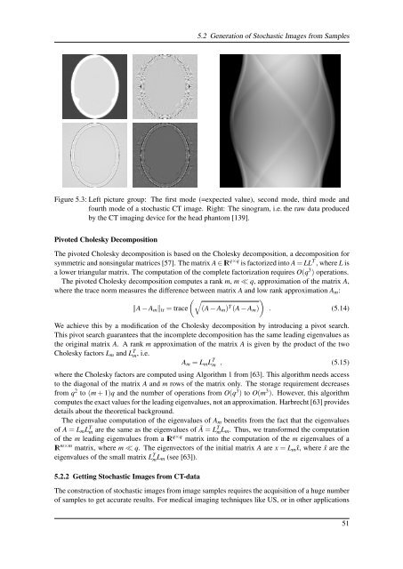
Figure 5.3: Left picture group: The first mode (=expected value), second mode, third mode and
fourth mode of a stochastic CT image. Right: The sinogram, i.e. the raw data produced
by the CT imaging device for the head phantom [139].
Pivoted Cholesky Decomposition
The pivoted Cholesky decomposition is based on the Cholesky decomposition, a decomposition for
symmetric and nonsingular matrices [57]. The matrix A ∈ IR q×q is factorized into A = LL T , where L is
a lower triangular matrix. The computation of the complete factorization requires O(q 3 ) operations.
The pivoted Cholesky decomposition computes a rank m, m ≪ q, approximation of the matrix A,
where the trace norm measures the difference between matrix A and low rank approximation A m :
(√
)
‖A − A m ‖ tr = trace (A − A m ) T (A − A m ) . (5.14)
We achieve this by a modification of the Cholesky decomposition by introducing a pivot search.
This pivot search guarantees that the incomplete decomposition has the same leading eigenvalues as
the original matrix A. A rank m approximation of the matrix A is given by the product of the two
Cholesky factors L m and L T m, i.e.
A m = L m L T m , (5.15)
where the Cholesky factors are computed using Algorithm 1 from [63]. This algorithm needs access
to the diagonal of the matrix A and m rows of the matrix only. The storage requirement decreases
from q 2 to (m + 1)q and the number of operations from O(q 3 ) to O(m 3 ). However, this algorithm
computes the exact values for the leading eigenvalues, not an approximation. Harbrecht [63] provides
details about the theoretical background.
The eigenvalue computation of the eigenvalues of A m benefits from the fact that the eigenvalues
of A = L m L T m are the same as the eigenvalues of à = L T mL m . Thus, we transformed the computation
of the m leading eigenvalues from a IR q×q matrix into the computation of the m eigenvalues of a
IR m×m matrix, where m ≪ q. The eigenvectors of the initial matrix A are x = L m ˆx, where ˆx are the
eigenvalues of the small matrix L T mL m (see [63]).
5.2.2 Getting Stochastic Images from CT-data
The construction of stochastic images from image samples requires the acquisition of a huge number
of samples to get accurate results. For medical imaging techniques like US, or in other applications
51