Segmentation of Stochastic Images using ... - Jacobs University

8.2 Ambrosio-Tortorelli Segmentation with Stochastic Parameters
8.2 Ambrosio-Tortorelli Segmentation with Stochastic Parameters
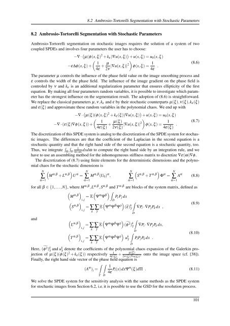
Ambrosio-Tortorelli segmentation on stochastic images requires the solution of a system of two
coupled SPDEs and involves four parameters the user has to choose:
−∇ · (µ(φ(x,ξ
) 2 + k ε )∇u(x,ξ ) ) + u(x,ξ ) = u 0 (x,ξ )
( 1
−ε∆φ(x,ξ ) +
4ε + µ )
2ν |∇u(x,ξ )|2 φ(x,ξ ) = 1
4ε . (8.6)
The parameter µ controls the influence of the phase field value on the image smoothing process and
ε controls the width of the phase field. The influence of the image gradient on the phase field is
controled by ν and k ε is an additional regularization parameter that ensures ellipticity of the first
equation. By making all four parameters random variables, it is possible to investigate which parameter
has the strongest influence on the segmentation result. The adoption of (8.6) is straightforward.
We replace the classical parameters µ,ν,k ε and ε by their stochastic counterparts µ(ξ ),ν(ξ ),k ε (ξ )
and ε(ξ ) and approximate these random variables in the polynomial chaos. We end up with
−∇ · (µ(ξ
)(φ(x,ξ ) 2 + k ε (ξ ))∇u(x,ξ ) ) + u(x,ξ ) = u 0 (x,ξ )
( 1
−∇ · (ε(ξ )∇φ(x,ξ )) +
4ε(ξ ) + µ(ξ ) )
2ν(ξ ) |∇u(x,ξ )|2 φ(x,ξ ) = 1
4ε(ξ ) . (8.7)
The discretization of this SPDE system is analog to the discretization of the SPDE system for stochastic
images. The differences are that the coefficient of the Laplacian in the second equation is a
stochastic quantity and that the right hand side of the second equation is a stochastic quantity, too.
∫D 1
4ε(ω)
Thus, we integrate ∫ Ω dxdω to compute the right hand side by an integration rule, and we
have to use an assembling method for the inhomogeneous stiffness matrix to discretize ∇ε(ω)∇φ.
The discretization of (8.7) using finite elements for the deterministic dimensions and the polynomial
chaos for the stochastic dimensions is
N
∑
α=1
(
) M α,β + L α,β U α =
N
∑
α=1
M α,β (U 0 ) α ,
N (
∑
α=1
S α,β + T α,β ) Φ α =
N
∑
α=1
A α (8.8)
for all β ∈ {1,...,N}, where M α,β ,L α,β ,S α,β and T α,β are blocks of the system matrix, defined as
(M ) (Ψ ) ∫
α,β = E α Ψ β P i P j dx
i, j D
( ) (
S α,β = ∑∑E
Ψ α Ψ β Ψ γ) ∫
(˜ε) k (8.9)
γ ∇P i · ∇P j P k dx ,
i, j
k γ
and (
(
L α,β ) i, j = ∑
k
T α,β ) i, j = ∑
k
(
∑E
γ
∑E
γ
Ψ α Ψ β Ψ γ) (˜φ 2 ) k γ
(
Ψ α Ψ β Ψ γ) u k γ
D
∫
D
∫
D
∇P i · ∇P j P k dx,
P i P j P k dx .
(8.10)
Here, (˜φ 2 ) k γ and u k γ denote the coefficients of the polynomial chaos expansion of the Galerkin projection
of µ(ξ )(φ(ξ ) 2 1
+ k ε (ξ )) respectively
4ε(ξ ) + µ(ξ )
onto the image space (cf. [38]).
2ν(ξ )|∇u(ξ )| 2
Finally, the right hand side vector of the phase field equation is
∫ ∫
(A α 1
) i =
4ε P i(x)dxΨ α (ξ )dΠ . (8.11)
Γ
D
We solve the SPDE system for the sensitivity analysis with the same methods as the SPDE system
for stochastic images from Section 6.2, i.e. it is possible to use the GSD for the resolution process.
101