

Segmentation of Stochastic Images using ... - Jacobs University
Segmentation of Stochastic Images using ... - Jacobs University
Segmentation of Stochastic Images using ... - Jacobs University

You also want an ePaper? Increase the reach of your titles
YUMPU automatically turns print PDFs into web optimized ePapers that Google loves.
3.3 Polynomial Chaos Expansions<br />
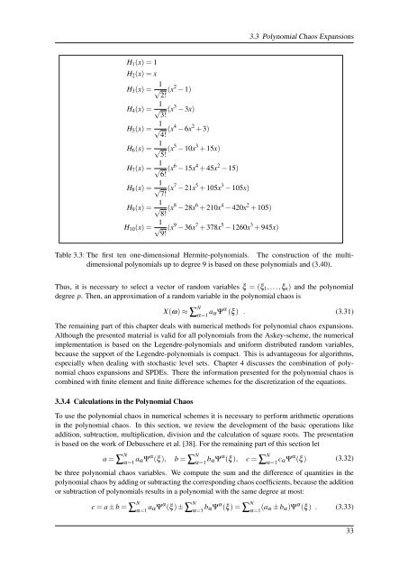
H 1 (x) = 1<br />
H 2 (x) = x<br />
H 3 (x) = 1 √<br />
2!<br />
(x 2 − 1)<br />
H 4 (x) = 1 √<br />
3!<br />
(x 3 − 3x)<br />
H 5 (x) = 1 √<br />
4!<br />
(x 4 − 6x 2 + 3)<br />
H 6 (x) = 1 √<br />
5!<br />
(x 5 − 10x 3 + 15x)<br />
H 7 (x) = 1 √<br />
6!<br />
(x 6 − 15x 4 + 45x 2 − 15)<br />
H 8 (x) = 1 √<br />
7!<br />
(x 7 − 21x 5 + 105x 3 − 105x)<br />
H 9 (x) = 1 √<br />
8!<br />
(x 8 − 28x 6 + 210x 4 − 420x 2 + 105)<br />
H 10 (x) = 1 √<br />
9!<br />
(x 9 − 36x 7 + 378x 5 − 1260x 3 + 945x)<br />
Table 3.3: The first ten one-dimensional Hermite-polynomials. The construction <strong>of</strong> the multidimensional<br />
polynomials up to degree 9 is based on these polynomials and (3.40).<br />
Thus, it is necessary to select a vector <strong>of</strong> random variables ξ = (ξ 1 ,...,ξ n ) and the polynomial<br />
degree p. Then, an approximation <strong>of</strong> a random variable in the polynomial chaos is<br />
X(ω) ≈ ∑ N α=1 a αΨ α (ξ ) . (3.31)<br />
The remaining part <strong>of</strong> this chapter deals with numerical methods for polynomial chaos expansions.<br />
Although the presented material is valid for all polynomials from the Askey-scheme, the numerical<br />
implementation is based on the Legendre-polynomials and uniform distributed random variables,<br />
because the support <strong>of</strong> the Legendre-polynomials is compact. This is advantageous for algorithms,<br />
especially when dealing with stochastic level sets. Chapter 4 discusses the combination <strong>of</strong> polynomial<br />
chaos expansions and SPDEs. There the information presented for the polynomial chaos is<br />
combined with finite element and finite difference schemes for the discretization <strong>of</strong> the equations.<br />
3.3.4 Calculations in the Polynomial Chaos<br />
To use the polynomial chaos in numerical schemes it is necessary to perform arithmetic operations<br />
in the polynomial chaos. In this section, we review the development <strong>of</strong> the basic operations like<br />
addition, subtraction, multiplication, division and the calculation <strong>of</strong> square roots. The presentation<br />
is based on the work <strong>of</strong> Debusschere et al. [38]. For the remaining part <strong>of</strong> this section let<br />
a = ∑ N α=1 a αΨ α (ξ ), b = ∑ N α=1 b αΨ α (ξ ), c = ∑ N α=1 c αΨ α (ξ ) (3.32)<br />
be three polynomial chaos variables. We compute the sum and the difference <strong>of</strong> quantities in the<br />
polynomial chaos by adding or subtracting the corresponding chaos coefficients, because the addition<br />
or subtraction <strong>of</strong> polynomials results in a polynomial with the same degree at most:<br />
c = a ± b = ∑ N α=1 a αΨ α (ξ ) ±∑ N α=1 b αΨ α (ξ ) = ∑ N α=1 (a α ± b α )Ψ α (ξ ) . (3.33)<br />
33


