Segmentation of Stochastic Images using ... - Jacobs University

4.4 Generalized Spectral Decomposition
functions are not fixed a priori. With the flexible basis functions we find a solution having significant
fewer modes, i.e. K ≪ N, but nearly the same approximation quality.
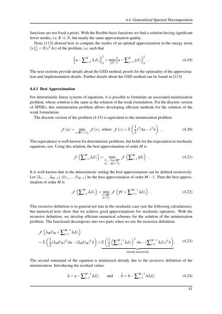
Nouy [113] showed how to compute the modes of an optimal approximation in the energy norm
‖v‖ 2 A = E(vT Av) of the problem, i.e. such that
∥
∥
∥u −∑ K ∥∥
j=1 λ 2
∥
jU j = min ∥
∥u −∑ K ∥∥
A γ,V
j=1 γ 2
jV j . (4.19)
A
The next sections provide details about the GSD method, proofs for the optimality of the approximation
and implementation details. Further details about the GSD method can be found in [113].
4.4.1 Best Approximation
For deterministic linear systems of equations, it is possible to formulate an associated minimization
problem, whose solution is the same as the solution of the weak formulation. For the discrete version
of SPDEs, this minimization problem allows developing efficient methods for the solution of the
weak formulation.
The discrete version of the problem (4.15) is equivalent to the minimization problem
( 1
J (u) = min J (v), where J (v) = E
v∈IR n ⊗S p 2 vT Au − v b)
T
. (4.20)
This equivalence is well-known for deterministic problems, but holds for the expectation in stochastic
equations, too. Using this relation, the best approximation of order M is
J
(
∑
M
i=1 λ iU i
)
( )
M
= min J
V 1 ,...V M ∈IR ∑ n i=1 γ iV i
γ i ,...,γ M ∈S p
. (4.21)
It is well-known that in the deterministic setting the best approximation can be defined recursively:
Let (λ 1 ,...,λ M−1 ),(U 1 ,...,U M−1 ) be the best approximation of order M − 1. Then the best approximation
of order M is
J
(
∑
M
i=1 λ iU i
)
(
)
= min J γV +∑ M−1
V ∈IR n
j=1 λ iU i
γ∈S p
. (4.22)
This recursive definition is in general not true in the stochastic case (see the following calculations),
but numerical tests show that we achieve good approximations for stochastic operators. With the
recursive definition, we develop efficient numerical schemes for the solution of the minimization
problem. The functional decomposes into two parts when we use the recursive definition:
(
λ M U M +∑ M−1
i=1 λ iU i
)
J
)
1
= E(
2 (λ MU M ) T Au − (λ M U M ) T b
( 1
(
M−1
+ E
2 ∑
)
i=1 λ iU i ) T b
i=1
) T λ iU i Au − ( ∑ M−1
} {{ }
already minimized
. (4.23)
The second summand of the equation is minimized already due to the recursive definition of the
minimization. Introducing the residual values
ũ = u −∑ M−1
i=1 λ iU i and ˜b = b − ∑ M−1
i=1 Aλ iU i (4.24)
41