Segmentation of Stochastic Images using ... - Jacobs University

5.4 Visualization of Stochastic Images
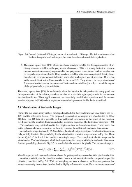
Figure 5.4: Second (left) and fifth (right) mode of a stochastic US image. The information encoded
in these images is hard to interpret, because there is no deterministic equivalent.
3. The ansatz space from [130] allows one basic random variable for the representation of arbitrary
random variables in the polynomial chaos only. This is a strong limitation, because
random variables reasonably representable in a polynomial chaos in one random variable can
be properly approximated only. Other random variables with more complicated density functions
have to be projected on this limited space, also leading to a loss of precision. This is due
to the double limit in the Cameron-Martin theorem [27]. They showed the approximation of
L 2 -random variables when the number of basic random variables ξ i ,i = 1,...,n and the degree
of the polynomials p goes to infinity.
The ansatz space from [130] is useful only when the solution is independent for every pixel and
the representation of the arbitrary random variable of a pixel through a polynomial in one random
variable is sufficient. These applications are rare, especially the diffusion equations used for demonstration
purposes in [130] and the segmentation methods presented in this thesis are critical.
5.4 Visualization of Stochastic Images
During the last years, many authors developed methods for the visualization of uncertainty, see [61,
125] and the references therein. The proposed visualization techniques are often limited to 1D or
2D data. For 1D data, it is possible to draw additional information in the graph of the function,
e.g. displaying the standard deviation and other stochastic quantities like kurtosis or skewness [125].
The stochastic images introduced in this chapter are two- or three-dimensional. Furthermore, due
to the polynomial chaos expansion, we have to visualize the additional stochastic dimensions.
A stochastic image is given by (5.3) and thus, the visualization techniques for classical images are
only partially feasible. One possibility for the visualization is via the images shown in Fig. 5.4. There
the set fα,i i ∈ I for fixed α is visualized as a single image. The complete stochastic image can be
visualized as N of such images, which is disappointing for images with high stochastic dimension.
Another possibility, shown in Fig. 5.5, is to calculate the variance for pixels. The variance image is
( ) (
f
i 2
α E (Ψ α (ξ )) 2) P i (x) . (5.17)
Var( f (x,ξ )) = ∑ i∈I ∑ N α=2
Visualizing expected value and variance allows for getting an impression about the pixels variability.
Another possibility for the visualization is to draw a set of samples from the computed output distribution,
visualized in Fig. 5.6. With this sampling, we look at classical, well-known, pictures, but
samples randomly drawn from the distribution highly influence the result. For a moderate number of
53