Segmentation of Stochastic Images using ... - Jacobs University

More documents

Recommendations

Info

Chapter 8 Segmentation of Classical Images Using Stochastic Parameters 8.1 Random Walker Segmentation with Stochastic Parameter The random walker segmentation has one free parameter that the user has to choose during the segmentation process. This parameter, denoted by β, controls the influence of the image gradient on the matrix entries because the edge weights for random walker segmentation (cf. Section 2.2) are ( w i j = exp −β (g i − g j ) 2) . (8.1) Making the parameter β a random variable and approximating this random variable in the polynomial chaos (cf. Section 3.3), the stochastic edge weights for the sensitivity analysis are w i j (ξ ) = exp ( − ( N∑ β α Ψ α (ξ ) α=1 )(g i − g j ) 2 ) . (8.2) Note that the parameter β is not restricted, but can be, the standard random variable for the construction of the polynomial chaos expansion, e.g. a uniform random variable. In fact, we use the power of the polynomial chaos approximation by making the parameter β dependent on a couple of standard random variables with an adequate polynomial degree in the polynomial chaos expansion. Using the stochastic edge weights from (8.2), we define the node degree analog to Section 6.1: d i (ξ ) = ∑ { j∈V :e i j ∈E} w i j (ξ ) = ∑ N ∑ { j∈V :e i j ∈E} α=1 (w i j ) α Ψ α (ξ ) . (8.3) Note that for the sensitivity analysis we use the exact normalization of the image gradient given by (2.6), because the pixel values are deterministic values in this setting. From the stochastic edge weights (8.2) and the stochastic node degrees (8.3), we construct the stochastic Laplacian matrix via ⎧ ⎨ L i j (ξ ) = ⎩ = N ∑ α=1 d i (ξ ) if i = j −w i j (ξ ) if v i and v j are adjacent nodes 0 otherwise L α Ψ α (ξ ) . Finally, we end up with the same stochastic equation system as in Section 6.1, but the stochastic components are due to the stochastic parameter instead of stochastic pixels inside the image: (8.4) L U (ξ )x U (ξ ) = −B(ξ ) T x M (ξ ) . (8.5) We have to use stochastic images to store the stochastic solution. The stochastic images have to contain the same random variables the parameter depends on. Remark 18. The discretization of the random walker segmentation with a stochastic parameter uses the generalized spectral decomposition. The only small variation in the implementation is that we have to use a polynomial chaos approximation of the parameter β for the calculation of the edge weights. The edge weights themselves are already random quantities in the stochastic random walker implementation of Section 6.1. 98
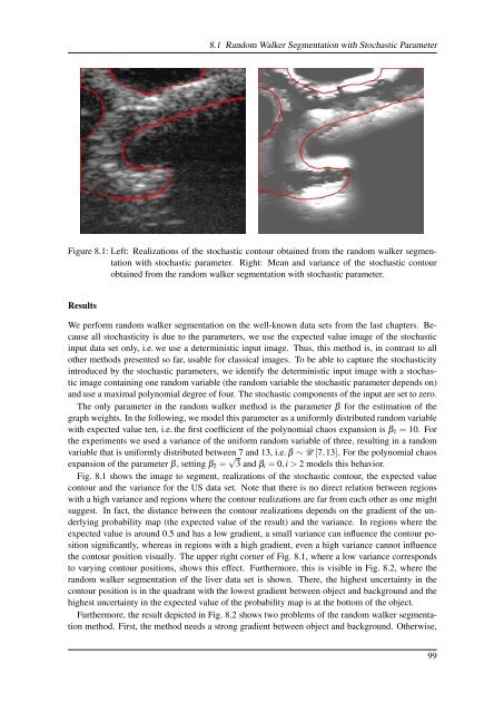
8.1 Random Walker Segmentation with Stochastic Parameter Figure 8.1: Left: Realizations of the stochastic contour obtained from the random walker segmentation with stochastic parameter. Right: Mean and variance of the stochastic contour obtained from the random walker segmentation with stochastic parameter. Results We perform random walker segmentation on the well-known data sets from the last chapters. Because all stochasticity is due to the parameters, we use the expected value image of the stochastic input data set only, i.e. we use a deterministic input image. Thus, this method is, in contrast to all other methods presented so far, usable for classical images. To be able to capture the stochasticity introduced by the stochastic parameters, we identify the deterministic input image with a stochastic image containing one random variable (the random variable the stochastic parameter depends on) and use a maximal polynomial degree of four. The stochastic components of the input are set to zero. The only parameter in the random walker method is the parameter β for the estimation of the graph weights. In the following, we model this parameter as a uniformly distributed random variable with expected value ten, i.e. the first coefficient of the polynomial chaos expansion is β 1 = 10. For the experiments we used a variance of the uniform random variable of three, resulting in a random variable that is uniformly distributed between 7 and 13, i.e. β ∼ U [7,13]. For the polynomial chaos expansion of the parameter β, setting β 2 = √ 3 and β i = 0,i > 2 models this behavior. Fig. 8.1 shows the image to segment, realizations of the stochastic contour, the expected value contour and the variance for the US data set. Note that there is no direct relation between regions with a high variance and regions where the contour realizations are far from each other as one might suggest. In fact, the distance between the contour realizations depends on the gradient of the underlying probability map (the expected value of the result) and the variance. In regions where the expected value is around 0.5 and has a low gradient, a small variance can influence the contour position significantly, whereas in regions with a high gradient, even a high variance cannot influence the contour position visually. The upper right corner of Fig. 8.1, where a low variance corresponds to varying contour positions, shows this effect. Furthermore, this is visible in Fig. 8.2, where the random walker segmentation of the liver data set is shown. There, the highest uncertainty in the contour position is in the quadrant with the lowest gradient between object and background and the highest uncertainty in the expected value of the probability map is at the bottom of the object. Furthermore, the result depicted in Fig. 8.2 shows two problems of the random walker segmentation method. First, the method needs a strong gradient between object and background. Otherwise, 99
Page 1:
Segmentation of Stochastic Images u
Page 5:
Abstract The task of segmentation,
Page 8 and 9:
7.5 Segmentation of Stochastic Imag
Page 11 and 12:
Chapter 1 Introduction The developm
Page 13 and 14:
Figure 1.3: This thesis combines fi
Page 15:
the presentation of the stochastic
Page 18 and 19:
Chapter 2 Image Segmentation and Li
Page 20 and 21:
Page 22 and 23:
Page 24 and 25:
Page 26 and 27:
Page 28 and 29:
Page 30 and 31:
Page 32 and 33:
Page 34 and 35:
Page 36 and 37:
Chapter 3 SPDEs and Polynomial Chao
Page 38 and 39:
Page 40 and 41:
Page 42 and 43:
Page 44 and 45:
Page 46 and 47:
Page 48 and 49:
Chapter 4 Discretization of SPDEs F
Page 50 and 51:
Chapter 4 Discretization of SPDEs 4
Page 52 and 53:
Chapter 4 Discretization of SPDEs a
Page 54 and 55:
Page 56 and 57:
Page 58 and 59: Chapter 5 Stochastic Images
Page 60 and 61: Chapter 5 Stochastic Images Figure
Page 62 and 63: Chapter 5 Stochastic Images like qu
Page 64 and 65: Chapter 5 Stochastic Images Figure
Page 67 and 68: Chapter 6 Segmentation of Stochasti
Page 69 and 70: 6.1 Random Walker Segmentation on S
Page 77 and 78: 6.2 Ambrosio-Tortorelli Segmentatio
Page 87: 6.2 Ambrosio-Tortorelli Segmentatio
Page 90 and 91: Chapter 7 Stochastic Level Sets whe
Page 92 and 93: Chapter 7 Stochastic Level Sets Fig
Page 94 and 95: Chapter 7 Stochastic Level Sets and
Page 96 and 97: Chapter 7 Stochastic Level Sets rar
Page 100 and 101: Chapter 7 Stochastic Level Sets MC
Page 106 and 107: Chapter 7 Stochastic Level Sets act
Page 110 and 111: Chapter 8 Segmentation of Classical
Page 118 and 119: Chapter 9 Summary, Discussion, and
Page 121 and 122: List of Figures 1.1 Left: CT image
Page 123 and 124: List of Figures 6.2 Mean and varian
Page 125: List of Figures 7.12 Mean (left) of
Page 129 and 130: Appendix A Publications Written Dur
Page 131 and 132: Bibliography [14] L. Ambrosio and M
Page 133 and 134: Bibliography [46] B. Echebarria, R.
Page 135 and 136: Bibliography [81] B. N. Khoromskij
Page 137 and 138: Bibliography [113] A. Nouy. A gener
Page 139: Bibliography [147] J. Tryoen, O. Le
show all

Segmentation of Stochastic Images using ... - Jacobs University

You also want an ePaper? Increase the reach of your titles

Delete template?

Save as template?