Segmentation of Stochastic Images using ... - Jacobs University

More documents

Recommendations

Info

Chapter 4 Discretization of SPDEs and performing an additional calculation for the first term results in ) 1 E( 2 (λ MU M ) T Au − (λ M U M ) T b ( 1 = E 2 (λ MU M ) T Aũ − (λ M U M ) T˜b 3 ( ) ) + 2 (λ MU M ) T M−1 A ∑ i=1 λ iU i . (4.25) In the deterministic case, the product (λ M U M ) T A ( ∑ M−1 i=1 λ ) iU i is equal to zero because Ui are eigenvectors of the operator A and therefore U ⊥ AU i . In the stochastic case, this is not true, but we neglect this small error. However, the numerical results are reasonable. We introduce a functional J ˜ : J ˜ 1 (λ M U M ) = E( 2 (λ MU M ) T Aũ − (λ M U M ) T˜b ) . (4.26) With the functional J ˜ , we transformed the minimization problem (4.20) into a series of simpler minimization problems. The next step is to find a method that allows an efficient solution of the problem series given by (4.26). Remark 6. The definition of the best approximation can be rewritten in matrix form as follows. Let W = (U 1 ,...,U M ) ∈ IR n×M be the matrix of all coefficients and Λ = (λ 1 ,...,λ M ) T ∈ IR M ⊗ S p the vector of stochastic functions. Then, (4.20) can equivalently be written J (WΛ) = min W∈IR n×M Λ∈IR M ⊗S p J (WΛ) , (4.27) and (4.26) can be written as ˜ J (U M λ M ) = min V ∈IR n γ∈IR⊗S p ˜ J (V γ) . (4.28) 4.4.2 Stationary Conditions for the Functionals J and J ˜ The simultaneous minimization of the functional J or J ˜ for deterministic W and stochastic Λ, respectively λ M and U M , is difficult due to the high dimension of the product space IR n ⊗ S p . A possibility to avoid the simultaneous minimization is to fix either the deterministic W or the stochastic Λ. For a fixed W, the stationary condition of J for Λ is and for fixed U the stationary condition of E ( Λ ∗T (W T AW)Λ ) = E ( Λ ∗T W T b ) ∀Λ ∗ ∈ IR M ⊗ S p , (4.29) ˜ J for λ is E ( λ ∗ (Ui T AU i )λ ) = E ( λ ∗ Ui T ˜b ) ∀λ ∗ ∈ S p . (4.30) Having the optimal Λ (or λ M ) at hand, we try to find a better W (or U M ) by solving stationary conditions for fixed Λ (or λ M ). For a fixed Λ, the stationary condition of J for W is and for fixed λ the stationary condition of E ( Λ T (W ∗T AW)Λ ) = E ( Λ T W ∗T b ) ∀W ∗ ∈ IR n×M , (4.31) E ( λ(U ∗T i ˜ J for U is AU i )λ ) = E ( λUi ∗T ˜b ) ∀U ∗ ∈ IR n . (4.32) Iterating these stationary conditions leads to a solution of the coupled problem (4.27). 42
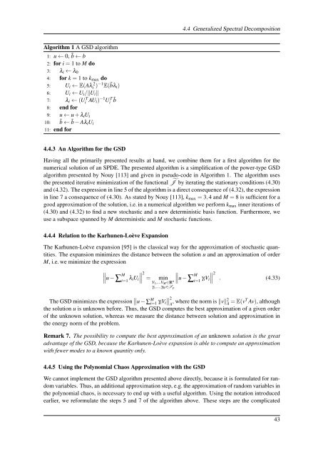
4.4 Generalized Spectral Decomposition Algorithm 1 A GSD algorithm 1: u ← 0, ˜b ← b 2: for i = 1 to M do 3: λ i ← λ 0 4: for k = 1 to k max do 5: U i ← E(Aλi 2)−1 E(˜bλ i ) 6: U i ← U i /‖U i ‖ 7: λ i ← (Ui T AU i ) −1 Ui T ˜b 8: end for 9: u ← u + λ i U i 10: ˜b ← ˜b − Aλ i U i 11: end for 4.4.3 An Algorithm for the GSD Having all the primarily presented results at hand, we combine them for a first algorithm for the numerical solution of an SPDE. The presented algorithm is a simplification of the power-type GSD algorithm presented by Nouy [113] and given in pseudo-code in Algorithm 1. The algorithm uses the presented iterative minimization of the functional J ˜ by iterating the stationary conditions (4.30) and (4.32). The expression in line 5 of the algorithm is a direct consequence of (4.32), the expression in line 7 a consequence of (4.30). As stated by Nouy [113], k max = 3,4 and M = 8 is sufficient for a good approximation of the solution, i.e. in a numerical algorithm we perform k max inner iterations of (4.30) and (4.32) to find a new stochastic and a new deterministic basis function. Furthermore, we use a subspace spanned by M deterministic and M stochastic functions. 4.4.4 Relation to the Karhunen-Loève Expansion The Karhunen-Loève expansion [95] is the classical way for the approximation of stochastic quantities. The expansion minimizes the distance between the solution u and an approximation of order M, i.e. we minimize the expression ∥ ∥u −∑ M i=1 λ iU i ∥ ∥∥ 2 = ∥ ∥ ∥∥u min − V 1 ,...V M ∑ M ∥∥ ∈IR n i=1 γ 2 iV i . (4.33) γ i ,...,γ M ∈S p The GSD minimizes the expression ∥ ∥u − ∑ M i=1 γ iV i ∥ ∥ 2 A , where the norm is ‖v‖2 A = E(vT Av), although the solution u is unknown before. Thus, the GSD computes the best approximation of a given order of the unknown solution, whereas we measure the distance between solution and approximation in the energy norm of the problem. Remark 7. The possibility to compute the best approximation of an unknown solution is the great advantage of the GSD, because the Karhunen-Loève expansion is able to compute an approximation with fewer modes to a known quantity only. 4.4.5 Using the Polynomial Chaos Approximation with the GSD We cannot implement the GSD algorithm presented above directly, because it is formulated for random variables. Thus, an additional approximation step, e.g. the approximation of random variables in the polynomial chaos, is necessary to end up with a useful algorithm. Using the notation introduced earlier, we reformulate the steps 5 and 7 of the algorithm above. These steps are the complicated 43
Page 1: Segmentation of Stochastic Images u
Page 5: Abstract The task of segmentation,
Page 8 and 9: 7.5 Segmentation of Stochastic Imag
Page 11 and 12: Chapter 1 Introduction The developm
Page 13 and 14: Figure 1.3: This thesis combines fi
Page 15: the presentation of the stochastic
Page 18 and 19: Chapter 2 Image Segmentation and Li
Page 36 and 37: Chapter 3 SPDEs and Polynomial Chao
Page 48 and 49: Chapter 4 Discretization of SPDEs F
Page 50 and 51: Chapter 4 Discretization of SPDEs 4
Page 58 and 59: Chapter 5 Stochastic Images
Page 60 and 61: Chapter 5 Stochastic Images Figure
Page 62 and 63: Chapter 5 Stochastic Images like qu
Page 64 and 65: Chapter 5 Stochastic Images Figure
Page 67 and 68: Chapter 6 Segmentation of Stochasti
Page 69 and 70: 6.1 Random Walker Segmentation on S
Page 77 and 78: 6.2 Ambrosio-Tortorelli Segmentatio
Page 87: 6.2 Ambrosio-Tortorelli Segmentatio
Page 90 and 91: Chapter 7 Stochastic Level Sets whe
Page 92 and 93: Chapter 7 Stochastic Level Sets Fig
Page 94 and 95: Chapter 7 Stochastic Level Sets and
Page 96 and 97: Chapter 7 Stochastic Level Sets rar
Page 98 and 99: Chapter 7 Stochastic Level Sets Fig
Page 100 and 101: Chapter 7 Stochastic Level Sets MC
Page 102 and 103:
Chapter 7 Stochastic Level Sets Fig
Page 104 and 105:
Chapter 7 Stochastic Level Sets Fig
Page 106 and 107:
Chapter 7 Stochastic Level Sets act
Page 108 and 109:
Chapter 8 Segmentation of Classical
Page 110 and 111:
Page 112 and 113:
Page 114 and 115:
Page 116 and 117:
Page 118 and 119:
Chapter 9 Summary, Discussion, and
Page 121 and 122:
List of Figures 1.1 Left: CT image
Page 123 and 124:
List of Figures 6.2 Mean and varian
Page 125:
List of Figures 7.12 Mean (left) of
Page 129 and 130:
Appendix A Publications Written Dur
Page 131 and 132:
Bibliography [14] L. Ambrosio and M
Page 133 and 134:
Bibliography [46] B. Echebarria, R.
Page 135 and 136:
Bibliography [81] B. N. Khoromskij
Page 137 and 138:
Bibliography [113] A. Nouy. A gener
Page 139:
Bibliography [147] J. Tryoen, O. Le
show all

Segmentation of Stochastic Images using ... - Jacobs University

You also want an ePaper? Increase the reach of your titles

Delete template?

Save as template?