Segmentation of Stochastic Images using ... - Jacobs University

4.5 Adaptive Grids
Figure 4.3: Refinement of a rectangular element of a finite element mesh. A single element on a
coarser level splits up into four elements on the next finer level.
4.5 Adaptive Grids
To improve the efficiency of the GSD further, we combine the GSD with an adaptive grid approach
for the spatial dimensions. Classically, images are represented by a regular grid, see Section 2.1.
The discretization of stochastic images using regular image grids and the polynomial chaos will be
described in detail in Section 5.1. Using adaptive grids for the spacial discretization we are able to use
an optimal small basis in the stochastic dimensions through the GSD and a minimal set of nodes in
the spatial dimensions, which reduces the memory requirements due to the tensor product structure.
We adopt the adaptive grid approach from [129], which is based on rectangular elements and a
quadtree structure for the refinement of the elements. Fig. 4.3 shows the refinement of a single
element. The main idea is to start on the finest grid level and to coarsen an element if the error
indicator S(x) of every node x of the element is smaller than a threshold ι.
As error indicator, we used the gradient of the expected value of the solution, i.e.
S(x) = |∇(E(u(x)))| . (4.39)
The adaptive coarsening of rectangular elements leads to constrained or hanging nodes, i.e. nodes
that are not vertices of all neighboring elements, see Fig. 4.4. These nodes need special handling
when we assemble the FE-matrices, because these nodes are not usual degrees of freedom. Instead,
they are constrained by the nodes which lie on the edges of the face the node lies on (see Fig. 4.4).
For details about the assembling of the FE-matrices with hanging nodes, we refer to [120, 129].
The error indicator S leads to problematic situations, in which the constraining node of a hanging
node is also a hanging node on the next coarser level. Fig. 4.5 shows such a situation. To avoid this,
the error indicator has to be saturated, as pointed out e.g. in [120, 129]. Following these references
the saturation condition is as follows.
Saturation condition. An error indicator value S(x) for x ∈ N (E) is always greater than every
error indicator S(x C ) for x C ∈ N C (E). In this formula, N (E) are the nodes of the element E and
N C (E) are the new nodes due to refinement of the element E.
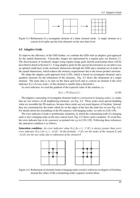
Figure 4.4: Refinement of elements leads to hanging nodes (circles) which are no degrees of freedom,
instead the values of the constraining nodes (squares) restrict them.
45