Segmentation of Stochastic Images using ... - Jacobs University

6.1 Random Walker Segmentation on Stochastic Images
Remark 9. The methods from Section 3.2 ensure existence and uniqueness for the solution of (6.7).
The coefficient fulfills w ∈ F l (D), because we use a truncated polynomial chaos representation.
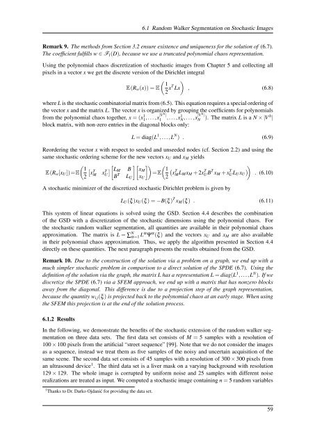
Using the polynomial chaos discretization of stochastic images from Chapter 5 and collecting all
pixels in a vector x we get the discrete version of the Dirichlet integral
) 1
E(R w (x)) = E(
2 xT Lx , (6.8)
where L is the stochastic combinatorial matrix from (6.5). This equation requires a special ordering of
the vector x and the matrix L. The vector x is organized by grouping the coefficients for polynomials
from the polynomial chaos together, x = (x1 1 h ,...,x|V |
1
,...,xN 1 h ,...,x|V |
N ). The matrix L is a N × |V h |
block matrix, with non-zero entries in the diagonal blocks only:
L = diag(L 1 ,...,L N ) . (6.9)
Reordering the vector x with respect to seeded and unseeded nodes (cf. Section 2.2) and using the
same stochastic ordering scheme for the new vectors x U and x M yields
( 1 [
E(R w [x U ])=E x
T
2 M xU] [ ][ ]) ( T L M B xM 1 (
B T
=E x
T
L U x U 2 M L M x M + 2xUB T T x M + xUL T ) )
U x U . (6.10)
A stochastic minimizer of the discretized stochastic Dirichlet problem is given by
L U (ξ )x U (ξ ) = −B(ξ ) T x M (ξ ) . (6.11)
This system of linear equations is solved using the GSD. Section 4.4 describes the combination
of the GSD with a discretization of the stochastic dimensions using the polynomial chaos. For
the stochastic random walker segmentation, all quantities are available in their polynomial chaos
approximation. The matrix is L = ∑ N α=1 Lα Ψ α (ξ ) and the vectors x U and x M are also available
in their polynomial chaos approximation. Thus, we apply the algorithm presented in Section 4.4
directly on these quantities. The next paragraph presents the results obtained from the GSD.
Remark 10. Due to the construction of the solution via a problem on a graph, we end up with a
much simpler stochastic problem in comparison to a direct solution of the SPDE (6.7). Using the
definition of the solution via the graph, the matrix L has a representation L = diag(L 1 ,...,L N ). If we
discretize the SPDE (6.7) via a SFEM approach, we end up with a matrix that has nonzero blocks
away from the diagonal. This difference is due to a projection step of the graph representation,
because the quantity w i j (ξ ) is projected back to the polynomial chaos at an early stage. When using
the SFEM this projection is at the end of the solution process.
6.1.2 Results
In the following, we demonstrate the benefits of the stochastic extension of the random walker segmentation
on three data sets. The first data set consists of M = 5 samples with a resolution of
100 × 100 pixels from the artificial “street sequence” [99]. Note that we do not consider the images
as a sequence, instead we treat them as five samples of the noisy and uncertain acquisition of the
same scene. The second data set consists of 45 samples with a resolution of 300 × 300 pixels from
an ultrasound device 1 . The third data set is a liver mask on a varying background with resolution
129 × 129. The whole image is corrupted by uniform noise and 25 samples with different noise
realizations are treated as input. We computed a stochastic image containing n = 5 random variables
1 Thanks to Dr. Darko Ojdanić for providing the data set.
59