Segmentation of Stochastic Images using ... - Jacobs University

Chapter 8 Segmentation of Classical Images Using Stochastic Parameters
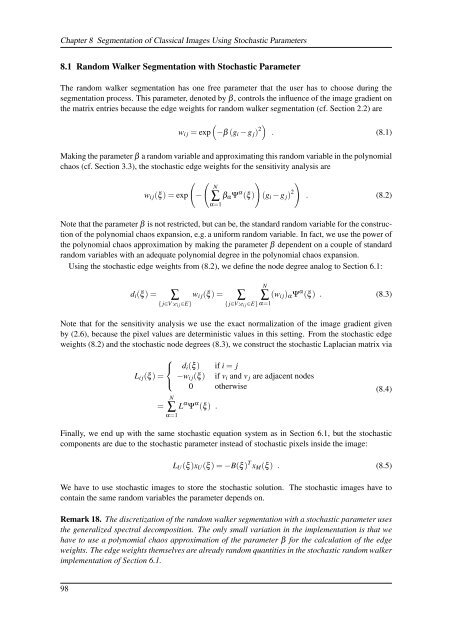
8.1 Random Walker Segmentation with Stochastic Parameter
The random walker segmentation has one free parameter that the user has to choose during the
segmentation process. This parameter, denoted by β, controls the influence of the image gradient on
the matrix entries because the edge weights for random walker segmentation (cf. Section 2.2) are
(
w i j = exp −β (g i − g j ) 2) . (8.1)
Making the parameter β a random variable and approximating this random variable in the polynomial
chaos (cf. Section 3.3), the stochastic edge weights for the sensitivity analysis are
w i j (ξ ) = exp
(
−
( N∑
β α Ψ α (ξ )
α=1
)(g i − g j ) 2 )
. (8.2)
Note that the parameter β is not restricted, but can be, the standard random variable for the construction
of the polynomial chaos expansion, e.g. a uniform random variable. In fact, we use the power of
the polynomial chaos approximation by making the parameter β dependent on a couple of standard
random variables with an adequate polynomial degree in the polynomial chaos expansion.
Using the stochastic edge weights from (8.2), we define the node degree analog to Section 6.1:
d i (ξ ) =
∑
{ j∈V :e i j ∈E}
w i j (ξ ) =
∑
N
∑
{ j∈V :e i j ∈E} α=1
(w i j ) α Ψ α (ξ ) . (8.3)
Note that for the sensitivity analysis we use the exact normalization of the image gradient given
by (2.6), because the pixel values are deterministic values in this setting. From the stochastic edge
weights (8.2) and the stochastic node degrees (8.3), we construct the stochastic Laplacian matrix via
⎧
⎨
L i j (ξ ) =
⎩
=
N
∑
α=1
d i (ξ ) if i = j
−w i j (ξ ) if v i and v j are adjacent nodes
0 otherwise
L α Ψ α (ξ ) .
Finally, we end up with the same stochastic equation system as in Section 6.1, but the stochastic
components are due to the stochastic parameter instead of stochastic pixels inside the image:
(8.4)
L U (ξ )x U (ξ ) = −B(ξ ) T x M (ξ ) . (8.5)
We have to use stochastic images to store the stochastic solution. The stochastic images have to
contain the same random variables the parameter depends on.
Remark 18. The discretization of the random walker segmentation with a stochastic parameter uses
the generalized spectral decomposition. The only small variation in the implementation is that we
have to use a polynomial chaos approximation of the parameter β for the calculation of the edge
weights. The edge weights themselves are already random quantities in the stochastic random walker
implementation of Section 6.1.
98