Segmentation of Stochastic Images using ... - Jacobs University

Chapter 6 Segmentation of Stochastic Images Using Elliptic SPDEs
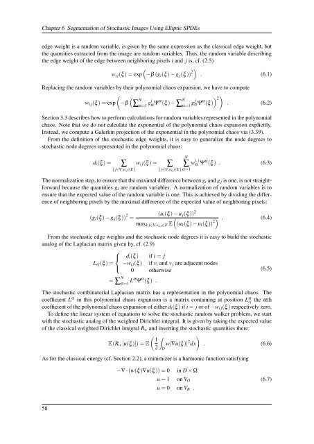
edge weight is a random variable, is given by the same expression as the classical edge weight, but
the quantities extracted from the image are random variables. Thus, the random variable describing
the edge weight of the edge between neighboring pixels i and j is, cf. (2.5)
(
w i j (ξ ) = exp −β (g i (ξ ) − g j (ξ )) 2) . (6.1)
Replacing the random variables by their polynomial chaos expansion, we have to compute
w i j (ξ ) = exp
( ( ) )
N
−β ∑ α=1 gi αΨ α (ξ ) −∑ N 2
α=1 g αΨ j α (ξ )
. (6.2)
Section 3.3 describes how to perform calculations for random variables represented in the polynomial
chaos. Note that we do not calculate the exponential of the polynomial chaos expansion explicitly.
Instead, we compute a Galerkin projection of the exponential in the polynomial chaos via (3.39).
From the definition of the stochastic edge weights, it is easy to generalize the node degrees to
stochastic node degrees represented in the polynomial chaos:
d i (ξ ) =
∑
{ j∈V :e i j ∈E}
w i j (ξ ) =
N
∑ ∑
{ j∈V :e i j ∈E} α=1
w i, j
α Ψ α (ξ ) . (6.3)
The normalization step, to ensure that the maximal difference between g i and g j is one, is not straightforward
because the quantities g i are random variables. A normalization of random variables is to
ensure that the expected value of the random variable is one. This is achieved by dividing the difference
of neighboring pixels by the maximal difference of the expected value of neighboring pixels:
(g i (ξ ) − g j (ξ )) 2 (u i (ξ ) − u j (ξ )) 2
=
. (6.4)
max k,l∈V,ek,l ∈E E
((u k (ξ ) − u l (ξ ))
2)
From the stochastic edge weights and the stochastic node degrees it is easy to build the stochastic
analog of the Laplacian matrix given by, cf. (2.9)
⎧
⎨ d i (ξ ) if i = j
L i j (ξ ) = −w i j (ξ ) if v i and v j are adjacent nodes
⎩
0 otherwise
(6.5)
= ∑ N α=1 Lα Ψ α (ξ ) .
The stochastic combinatorial Laplacian matrix has a representation in the polynomial chaos. The
coefficient L α in this polynomial chaos expansion is a matrix containing at position Li α j the αth
coefficient of the polynomial chaos expansion of either d i (ξ ) if i = j or of −w i j (ξ ) respectively zero.
To define the linear system of equations to solve the stochastic random walker problem, we start
with the stochastic analog of the weighted Dirichlet integral. It is given by taking the expected value
of the classical weighted Dirichlet integral R w and inserting the stochastic quantities there:
( ∫
)
1
E(R w [u(ξ )]) = E w|∇u(ξ )| 2 dx . (6.6)
2 D
As for the classical energy (cf. Section 2.2), a minimizer is a harmonic function satisfying
−∇ · (w(ξ )∇u(ξ )) = 0 in D × Ω
u = 1 on V O
u = 0 on V B .
(6.7)
58