Segmentation of Stochastic Images using ... - Jacobs University

Chapter 6 Segmentation of Stochastic Images Using Elliptic SPDEs
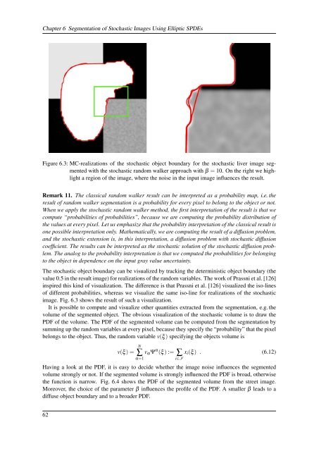
Figure 6.3: MC-realizations of the stochastic object boundary for the stochastic liver image segmented
with the stochastic random walker approach with β = 10. On the right we highlight
a region of the image, where the noise in the input image influences the result.
Remark 11. The classical random walker result can be interpreted as a probability map, i.e. the
result of random walker segmentation is a probability for every pixel to belong to the object or not.
When we apply the stochastic random walker method, the first interpretation of the result is that we
compute “probabilities of probabilities”, because we are computing the probability distribution of
the values at every pixel. Let us emphasize that the probability interpretation of the classical result is
one possible interpretation only. Mathematically, we are computing the result of a diffusion problem,
and the stochastic extension is, in this interpretation, a diffusion problem with stochastic diffusion
coefficient. The results can be interpreted as the stochastic solution of the stochastic diffusion problem.
The analog to the probability interpretation is that we computed the probabilities for belonging
to the object in dependence on the input gray value uncertainty.
The stochastic object boundary can be visualized by tracking the deterministic object boundary (the
value 0.5 in the result image) for realizations of the random variables. The work of Prassni et al. [126]
inspired this kind of visualization. The difference is that Prassni et al. [126] visualized the iso-lines
of different probabilities, whereas we visualize the same iso-line for realizations of the stochastic
image. Fig. 6.3 shows the result of such a visualization.
It is possible to compute and visualize other quantities extracted from the segmentation, e.g. the
volume of the segmented object. The obvious visualization of the stochastic volume is to draw the
PDF of the volume. The PDF of the segmented volume can be computed from the segmentation by
summing up the random variables at every pixel, because they specify the “probability” that the pixel
belongs to the object. Thus, the random variable v(ξ ) specifying the objects volume is
v(ξ ) =
N
∑
α=1
v α Ψ α (ξ ) := ∑ x i (ξ ) . (6.12)
i∈I
Having a look at the PDF, it is easy to decide whether the image noise influences the segmented
volume strongly or not. If the segmented volume is strongly influenced the PDF is broad, otherwise
the function is narrow. Fig. 6.4 shows the PDF of the segmented volume from the street image.
Moreover, the choice of the parameter β influences the profile of the PDF. A smaller β leads to a
diffuse object boundary and to a broader PDF.
62