Segmentation of Stochastic Images using ... - Jacobs University

More documents

Recommendations

Info

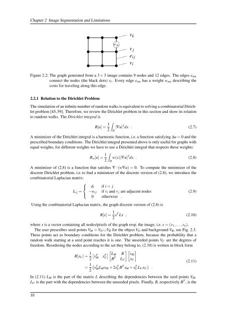
Chapter 2 Image Segmentation and Limitations ✈ ✈ ✈ ✈ ✈ ✈ ✈✘ ✘ ✘ v k ✎☞ w 7 ✍✌ jk ✘✘✘ ✈ v j ✘ ✘ ✘ e i j ✘✈ ✘ ✘ v i Figure 2.2: The graph generated from a 3 × 3 image contains 9 nodes and 12 edges. The edges e mn connect the nodes (the black dots) v l . Every edge e mn has a weight w mn describing the costs for traveling along this edge. 2.2.1 Relation to the Dirichlet Problem The simulation of an infinite number of random walks is equivalent to solving a combinatorial Dirichlet problem [45,59]. Therefore, we review the Dirichlet problem in this section and show its relation to random walks. The Dirichlet integral is R[u] = 1 ∫ |∇u| 2 dx . (2.7) 2 D A minimizer of the Dirichlet integral is a harmonic function, i.e. a function satisfying ∆u = 0 and the prescribed boundary conditions. The Dirichlet integral presented above is only useful for graphs with equal weights, for different weights we have to use a Dirichlet integral that respects these weights: R w [u] = 1 ∫ w(x)|∇u| 2 dx . (2.8) 2 D A minimizer of (2.8) is a function that satisfies ∇ · (w∇u) = 0. To compute the minimizer of the discrete Dirichlet problem, i.e. to find a minimizer of the discrete version of (2.8), we introduce the combinatorial Laplacian matrix: ⎧ ⎨ d i if i = j L i j = −w i j if v i and v j are adjacent nodes (2.9) ⎩ 0 otherwise . Using the combinatorial Laplacian matrix, the graph discrete version of (2.8) is R[x] = 1 2 xT Lx , (2.10) where x is a vector containing all nodes/pixels of the graph resp. the image, i.e. x = (v 1 ,...,v n ). The user prescribes seed points V M = V O ∪V B for the object V O and background V B , see Fig. 2.3. These points act as boundary conditions for the Dirichlet problem, because the probability that a random walk starting at a seed point reaches it is one. The unseeded points V U are the degrees of freedom. Reordering the nodes according to the set they belong to, (2.10) is written in block form R[x U ] = 1 [ x T 2 M xU] [ ][ ] T L M B xM B T L U x U = 1 (2.11) ( x T 2 M L M x M + 2xUB T T x M + xUL T ) U x U . In (2.11) L M is the part of the matrix L describing the dependencies between the seed points V M . L U is the part with the dependencies between the unseeded pixels. Finally, B, respectively B T , is the 10
2.2 Random Walker Segmentation Figure 2.3: Left: Definition of the seed regions for the object (yellow) and the background (red). Middle: The probability that a random walker reaches an object seed. Black denotes probability zero, white probability one. Right: Random walker segmentation result of the ultrasound image. As input we used the seed regions from the left image and β = 200. part of the matrix describing the coupling between the seeded and unseeded pixels. Differentiation of (2.11) yields a minimizer of (2.11) given by the solution of L U x U = −B T x M . (2.12) Remark 2. For 2D-images, the matrices L U and B are band matrices with five bands used only. The numerical solution of the system benefits from the use of numerical methods that make use of this special matrix structure, e.g. , it is necessary to store five bands as single vectors only. Furthermore, arithmetic operations for matrices with band structure can be implemented efficiently [57]. As already mentioned, the random walker segmentation is an interactive segmentation method. Due to the fast calculation of the random walker result, the user interactively defines new seed regions or eliminates unwanted seed regions to get an optimal segmentation result. Fig. 2.4 shows three steps of the computer/user interaction for the refinement of a segmentation result. Another, more mathematical, motivation for the derivation of (2.12) is that we have to solve −∇ · (w∇u) = 0 in D u = 1 on V O u = 0 on V B . (2.13) Transforming this PDE to homogeneous boundary conditions [124], applying the reordering of the nodes, and using the combinatorial Laplacian, we end up with (2.12). Eq. (2.12) is a system of linear equations solvable by using iterative methods, e.g. the method of conjugate gradients. Remark 3. The presented segmentation method, the random walker segmentation, sounds like a stochastic method for segmentation that includes randomness and uncertainty, but this is false. Using the equivalence to the Dirichlet problem presented above, the method computes deterministic weights for an elliptic PDE on a graph. Thus, all “randomness” is lost. The “randomness” comes from the interpretation of the result: Every pixel gets a value between zero and one, and we interpret these values as probabilities for reaching the seed region from this specific pixel. The random walker segmentation result is a probability for every pixel for belonging to the object (see middle of Fig. 2.3). Typically, the threshold 0.5 distinguishes between the object and the background. A pixel having a probability above 50% is assigned to the object and a pixel with a probability below 50% to the background. Fig. 2.3 shows a random walker segmentation result. 11
Page 1: Segmentation of Stochastic Images u
Page 5: Abstract The task of segmentation,
Page 8 and 9: 7.5 Segmentation of Stochastic Imag
Page 11 and 12: Chapter 1 Introduction The developm
Page 13 and 14: Figure 1.3: This thesis combines fi
Page 15: the presentation of the stochastic
Page 18 and 19: Chapter 2 Image Segmentation and Li
Page 36 and 37: Chapter 3 SPDEs and Polynomial Chao
Page 48 and 49: Chapter 4 Discretization of SPDEs F
Page 50 and 51: Chapter 4 Discretization of SPDEs 4
Page 52 and 53: Chapter 4 Discretization of SPDEs a
Page 58 and 59: Chapter 5 Stochastic Images
Page 60 and 61: Chapter 5 Stochastic Images Figure
Page 62 and 63: Chapter 5 Stochastic Images like qu
Page 64 and 65: Chapter 5 Stochastic Images Figure
Page 67 and 68: Chapter 6 Segmentation of Stochasti
Page 69 and 70: 6.1 Random Walker Segmentation on S
Page 71 and 72:
6.1 Random Walker Segmentation on S
Page 73 and 74:
Page 75 and 76:
Page 77 and 78:
6.2 Ambrosio-Tortorelli Segmentatio
Page 79 and 80:
Page 81 and 82:
Page 83 and 84:
Page 85 and 86:
Page 87:
Page 90 and 91:
Chapter 7 Stochastic Level Sets whe
Page 92 and 93:
Chapter 7 Stochastic Level Sets Fig
Page 94 and 95:
Chapter 7 Stochastic Level Sets and
Page 96 and 97:
Chapter 7 Stochastic Level Sets rar
Page 98 and 99:
Page 100 and 101:
Chapter 7 Stochastic Level Sets MC
Page 102 and 103:
Page 104 and 105:
Page 106 and 107:
Chapter 7 Stochastic Level Sets act
Page 108 and 109:
Chapter 8 Segmentation of Classical
Page 110 and 111:
Page 112 and 113:
Page 114 and 115:
Page 116 and 117:
Page 118 and 119:
Chapter 9 Summary, Discussion, and
Page 121 and 122:
List of Figures 1.1 Left: CT image
Page 123 and 124:
List of Figures 6.2 Mean and varian
Page 125:
List of Figures 7.12 Mean (left) of
Page 129 and 130:
Appendix A Publications Written Dur
Page 131 and 132:
Bibliography [14] L. Ambrosio and M
Page 133 and 134:
Bibliography [46] B. Echebarria, R.
Page 135 and 136:
Bibliography [81] B. N. Khoromskij
Page 137 and 138:
Bibliography [113] A. Nouy. A gener
Page 139:
Bibliography [147] J. Tryoen, O. Le
show all

Segmentation of Stochastic Images using ... - Jacobs University

You also want an ePaper? Increase the reach of your titles

Delete template?

Save as template?