Segmentation of Stochastic Images using ... - Jacobs University

Chapter 3 SPDEs and Polynomial Chaos Expansions
H 1 (x) = 1
H 2 (x) = √ 3x
H 3 (x) = √ 5 · (1.5 ∗ x 2 − 0.5)
H 4 (x) = √ 7 · (2.5x 3 − 1.5 ∗ x)
H 5 (x) = √ 9 · 1
8 (35x4 − 30x 2 + 3.0)
H 6 (x) = √ 11 · 1
8 (63x5 − 70x 3 + 15x)
H 7 (x) = √ 13 · 1
16 (231x6 − 315x 4 + 105x − 5)
H 8 (x) = √ 15 · 1
16 (429x7 − 693x 5 + 315x 3 − 35x)
H 9 (x) = √ 1
17 ·
128 (6435x8 − 12012x 6 + 6930x 4 − 1260x 2 + 35)
H 10 (x) = √ 1
19 ·
128 (12155x9 − 25740x 7 + 18018x 5 − 4620x 3 + 315x)
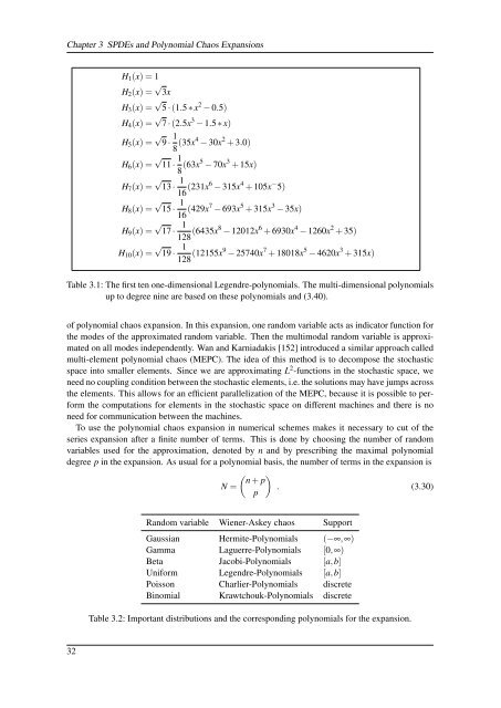
Table 3.1: The first ten one-dimensional Legendre-polynomials. The multi-dimensional polynomials
up to degree nine are based on these polynomials and (3.40).
of polynomial chaos expansion. In this expansion, one random variable acts as indicator function for
the modes of the approximated random variable. Then the multimodal random variable is approximated
on all modes independently. Wan and Karniadakis [152] introduced a similar approach called
multi-element polynomial chaos (MEPC). The idea of this method is to decompose the stochastic
space into smaller elements. Since we are approximating L 2 -functions in the stochastic space, we
need no coupling condition between the stochastic elements, i.e. the solutions may have jumps across
the elements. This allows for an efficient parallelization of the MEPC, because it is possible to perform
the computations for elements in the stochastic space on different machines and there is no
need for communication between the machines.
To use the polynomial chaos expansion in numerical schemes makes it necessary to cut of the
series expansion after a finite number of terms. This is done by choosing the number of random
variables used for the approximation, denoted by n and by prescribing the maximal polynomial
degree p in the expansion. As usual for a polynomial basis, the number of terms in the expansion is
( ) n + p
N = . (3.30)
p
Random variable Wiener-Askey chaos Support
Gaussian Hermite-Polynomials (−∞,∞)
Gamma Laguerre-Polynomials [0,∞)
Beta Jacobi-Polynomials [a,b]
Uniform Legendre-Polynomials [a,b]
Poisson Charlier-Polynomials discrete
Binomial Krawtchouk-Polynomials discrete
Table 3.2: Important distributions and the corresponding polynomials for the expansion.
32