Segmentation of Stochastic Images using ... - Jacobs University

More documents

Recommendations

Info

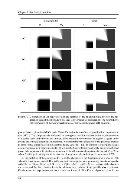
Chapter 7 Stochastic Level Sets rarefaction fan shock E Var E Var PC SC MC MCL Figure 7.3: Comparison of the expected value and variance of the resulting phase field for the rarefaction fan and the shock, two classical tests for level set propagation. The figure shows the comparison of the four discretizations of the stochastic phase field equation. preconditioned phase field (MC), and a Monte Carlo simulation of the original level set implementation (MCL). The comparison is performed on two typical tests for level set evolution, the evolution of a cosine curve in the inward and outward direction and the evolution of an edge of a square in the inward and outward direction. Furthermore, we demonstrate the extension of the proposed method to three spatial dimensions on the Stanford bunny data set [149]. In contrast to other publications dealing with mean curvature motion [138], we use the Stanford bunny and apply the preconditioned phase field equation with stochastic speed on it. In all numerical experiments, we set W = 2.5h, where h is the grid spacing and in the absence of a curvature dependent speed, we set b = 1.25h. For the evolution of the cosine (see Fig. 7.2), the challenge is the development of a shock [138], when the curve moves inward. Due to the stochastic velocity, we used a uniformly distributed speed a with E(a) = 1.0 and Var(a) = 0.04, i.e. a ∼ U [1 − 0.2 √ 3,1 + 0.2 √ 3], the position of the shock is uncertain, and the discretization has to be adequate in a vicinity of the possible shock positions. For the numerical experiments, we use a spatial resolution of 129 × 129, a polynomial chaos in one 86
7.4 Numerical Experiments Figure 7.4: Expected value color-coded by the variance for the Stanford bunny after shrinkage under an uncertain speed in the normal direction. Red indicates regions with a high variance and green regions with low variance. In addition, we show one slice of the variance. random variable with order two and apply 30 steps with step size 0.1h. Furthermore, we computed 20 time steps of the reinitialization equation (7.24) with step size 0.2h after every time step. The polynomial chaos coefficients of the speed are set to a 1 = 1, a 2 = 0.2, and a 3 = 0, such that the expansion fulfills E(a) = 1 and Var(a) = 0.04. It is visible from Fig. 7.2 that the methods based on the stochastic preconditioned phase field formulation lead to the same results. Only the discretization of the level set method leads to deviating results. This is due to the reinitialization of the level set via Fast Marching [138]. The Fast Marching method assumes that the level set values at a grid point near the interface, the trial nodes (see [138]) is the signed distance to the interface. This is not true in the presence of a shock due to the crossing of the zero level set. For deterministic level sets this error can be neglected, even for stochastic level sets the expected value is accurate. However, for the stochastic part of the solution (the variance in Fig. 7.2), which is orders of magnitude smaller than the expected value, this error becomes relevant. Thus, it is more precise to use the reinitialization via (7.24) in the presence of a shock. When the interface moves outward, we have a rarefaction fan (see [138]), because one point on the zero level set is the closest point for multiple points away from the interface. The same problem as for the shock arises and again, the reinitialization via (7.24) is the better method. The second test is the evolution of one edge of a square in the inward and outward direction depicted in Fig. 7.3. Again, we have the development of a shock when the curve moves inward and of a rarefaction fan when the curve moves outward. The last test is the contraction of the Stanford bunny under an uncertain velocity. Again, we used the speed E(a) = 1.0 and Var(a) = 0.04 from the previous tests. Fig. 7.4 shows the results. For the Stanford bunny, we have the evolution of a 3D object. We use a method for the visualization of 3D stochastic images from Section 5.4 by visualizing the expected value color-coded by the variance. As expected, we see a high variance of the contour in regions with high curvature. This is due to the development of shocks, when the contour moves inside these regions. 87
Page 1:
Segmentation of Stochastic Images u
Page 5:
Abstract The task of segmentation,
Page 8 and 9:
7.5 Segmentation of Stochastic Imag
Page 11 and 12:
Chapter 1 Introduction The developm
Page 13 and 14:
Figure 1.3: This thesis combines fi
Page 15:
the presentation of the stochastic
Page 18 and 19:
Chapter 2 Image Segmentation and Li
Page 20 and 21:
Page 22 and 23:
Page 24 and 25:
Page 26 and 27:
Page 28 and 29:
Page 30 and 31:
Page 32 and 33:
Page 34 and 35:
Page 36 and 37:
Chapter 3 SPDEs and Polynomial Chao
Page 38 and 39:
Page 40 and 41:
Page 42 and 43:
Page 44 and 45:
Page 46 and 47: Chapter 3 SPDEs and Polynomial Chao
Page 48 and 49: Chapter 4 Discretization of SPDEs F
Page 50 and 51: Chapter 4 Discretization of SPDEs 4
Page 52 and 53: Chapter 4 Discretization of SPDEs a
Page 58 and 59: Chapter 5 Stochastic Images
Page 60 and 61: Chapter 5 Stochastic Images Figure
Page 62 and 63: Chapter 5 Stochastic Images like qu
Page 64 and 65: Chapter 5 Stochastic Images Figure
Page 67 and 68: Chapter 6 Segmentation of Stochasti
Page 69 and 70: 6.1 Random Walker Segmentation on S
Page 77 and 78: 6.2 Ambrosio-Tortorelli Segmentatio
Page 87: 6.2 Ambrosio-Tortorelli Segmentatio
Page 90 and 91: Chapter 7 Stochastic Level Sets whe
Page 92 and 93: Chapter 7 Stochastic Level Sets Fig
Page 94 and 95: Chapter 7 Stochastic Level Sets and
Page 100 and 101: Chapter 7 Stochastic Level Sets MC
Page 106 and 107: Chapter 7 Stochastic Level Sets act
Page 108 and 109: Chapter 8 Segmentation of Classical
Page 118 and 119: Chapter 9 Summary, Discussion, and
Page 121 and 122: List of Figures 1.1 Left: CT image
Page 123 and 124: List of Figures 6.2 Mean and varian
Page 125: List of Figures 7.12 Mean (left) of
Page 129 and 130: Appendix A Publications Written Dur
Page 131 and 132: Bibliography [14] L. Ambrosio and M
Page 133 and 134: Bibliography [46] B. Echebarria, R.
Page 135 and 136: Bibliography [81] B. N. Khoromskij
Page 137 and 138: Bibliography [113] A. Nouy. A gener
Page 139: Bibliography [147] J. Tryoen, O. Le
show all

Segmentation of Stochastic Images using ... - Jacobs University

You also want an ePaper? Increase the reach of your titles

Delete template?

Save as template?