Segmentation of Stochastic Images using ... - Jacobs University

8.4 Geodesic Active Contours with Stochastic Parameters
8.4 Geodesic Active Contours with Stochastic Parameters
The sensitivity analysis for the geodesic active contour approach follows the procedure for the sensitivity
analysis of the other segmentation methods. Geodesic active contours are given by
φ t (t,x) = γg(t,x)κ(t,x)|∇φ(t,x)| + α∇g(t,x)∇φ(t,x) − βg|∇φ| . (8.13)
The parameters α,β, and γ can be chosen to optimize the segmentation result. The parameter α
controls the attraction of the minima of the speed function v. The parameter β controls the shrinkage
(negative β) or expansion (positive β) of the level set and the parameter γ acts as a weighting term
for the curvature smoothing.
Making the segmentation parameters random variables, we end up with
φ t = γ(ω)g(t,x,ω)κ(t,x,ω)|∇φ(t,x,ω)| + α(ω)∇g(t,x,ω)∇φ(t,x,ω) − β(ω)g|∇φ| . (8.14)
This equation is nearly identical to the stochastic geodesic active contour equation, but requires an
additional projection step during the discretization to projects the products γg,α∇g, and βg back to
the polynomial chaos. Besides this additional projection step, we use the same numerical methods
as for the discretization of the stochastic geodesic active contour equation in Section 7.5.2, i.e. we
use an explicit time step discretization via the Euler method and a uniform spatial grid.
Results
The geodesic active contour method with stochastic parameters is performed on the same data sets as
in the previous sections. Due to the smooth objects that we try to segment in the images, we ignore
the smoothing term by setting γ = 0. The parabolic approximation and the attraction term ∇g∇φ
ensure that we get smooth results in this setting, too. The parameters α and β are chosen by setting
α 1 = 0.08, α 2 = 0.002, β 1 = 1.0, and β 2 = 0.02. Thus, we use two stochastic parameters at the same
time and make them both dependent on the same random variable. Since we set the expected value
and the first coefficient to a nonzero value, we end up with uniformly distributed parameters.
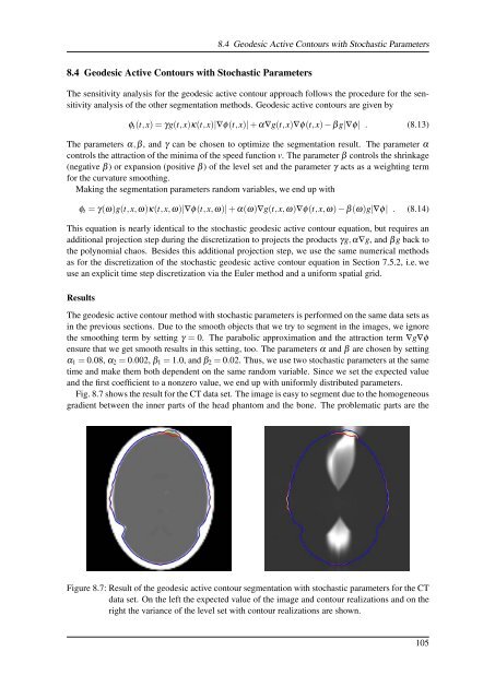
Fig. 8.7 shows the result for the CT data set. The image is easy to segment due to the homogeneous
gradient between the inner parts of the head phantom and the bone. The problematic parts are the
Figure 8.7: Result of the geodesic active contour segmentation with stochastic parameters for the CT
data set. On the left the expected value of the image and contour realizations and on the
right the variance of the level set with contour realizations are shown.
105