Segmentation of Stochastic Images using ... - Jacobs University

Chapter 2 Image Segmentation and Limitations
✘ ✘✘ ✘ ✘✘✘ u(x j ) = u j
✘ ✘ ✘ ✘✘ ✘ ✘ x i
❳ ❳❳
❳ ❳ ❳
supp Pi (x)
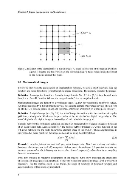
Figure 2.1: Sketch of the ingredients of a digital image. At every intersection of the regular grid lines
a pixel is located and for every pixel the corresponding FE basis function has its support
in the elements around this pixel.
2.1 Mathematical Images
Before we start with the presentation of segmentation methods, we give a short overview over the
notation and basic definitions for mathematical image processing. The primary object is the image:
Definition An image is a function u from the image domain D ⊂ IR d ,d ∈ {2,3}, into the real numbers,
i.e. u : D → IR. In what follows, the image domain D is a rectangular domain.
Mathematical images are defined on a continuous space, i.e. they have an infinite number of values.
An image acquired by a digital imaging device, e.g. a digital camera or advanced devices like CT [66]
or MR [91], is called a digital image and the image intensities are known on a finite point set only:
Definition A digital image (see Fig. 2.1) is a set of image intensities at the intersections of regular
grid lines, called pixels. We denote the pixel value of the ith pixel of the digital image u by u i . The
set of all pixels of a digital image is denoted by I and called the image grid.
The link between this continuous definition and the pixel representation of digital images is the usage
of an interpolation rule. Let us denote by P i the bilinear (2D) or trilinear (3D), basis function of the
i-th pixel belonging to the multi-linear finite element space of the grid I . Then a digital image is
interpolated at every point x in the image domain D by using the interpolation
u(x) = ∑ u i P i (x) . (2.1)
i∈I
Remark 1. In what follows, we deal with gray value images only. This is not a strong restriction,
because color images are typically composed of three color channels and it is possible to apply the
methods presented in the following on these color channels separately when there is no coupling
between the channels.
Until now, we have no regularity assumptions on the image u, but to show existence and uniqueness
of solutions of image processing methods, we have to restrict the analysis to images with a prescribed
regularity. For the methods used in this thesis, the space of functions of bounded variation and
generalizations of this space are important.
8