Segmentation of Stochastic Images using ... - Jacobs University

Chapter 5 Stochastic Images
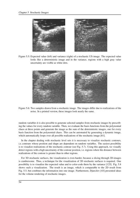
Figure 5.5: Expected value (left) and variance (right) of a stochastic US-image. The expected value
looks like a deterministic image and in the variance, regions with a high gray value
uncertainty are visible as white dots.
Figure 5.6: Two samples drawn from a stochastic image. The images differ due to realizations of the
noise. In a printed version, these images look nearly the same.
random variables it is also possible to generate selected samples from stochastic images by prescribing
the values for every random variable. Then, we evaluate the basis functions from the polynomial
chaos at these points and generate the image as the sum of the deterministic images, one for every
basis function from the polynomial chaos. This can be automated by generating a dynamic image,
which automatically loops over all possible realizations of the stochastic image [61].
In the chapter dealing with stochastic level sets it is necessary to visualize stochastic contours,
i.e. contours whose position and shape are dependent on random variables. The easiest possibility
is to visualize realizations of the stochastic contour (see Fig. 5.7). Using this approach, we visually
detect regions with a high uncertainty of the contour position, i.e. regions where the distance between
realizations of the contour is greater than in other regions.
For 3D stochastic surfaces, the visualization is even harder, because a slicing through 2D-images
is cumbersome. Thus, a technique for the visualization of 3D stochastic surfaces is required. One
possibility is to visualize the expected value and to color-code them by the variance [125]. Fig. 5.8
shows such a visualization. The result is an image, which is comparable to the 2D result from
Fig. 5.5, but combines the information into one image. Furthermore, Djurcilov [43] presented ideas
for the volume rendering of stochastic images.
54