Segmentation of Stochastic Images using ... - Jacobs University

More documents

Recommendations

Info

Chapter 3 SPDEs and Polynomial Chaos Expansions Roughly speaking, a Kondratiev space S ρ,k is a subspace of L 2 (Ω), where the coefficients f α respect a decay condition such that (3.13) stays finite. The Kondratiev spaces from the previous definition are purely stochastic spaces. To add the spatial dependencies we have to make the coefficients f α functions that depend on a spatial variable and fulfill regularity assumptions. Definition The Hilbert space (S ) ρ,k,m (D) is { } (S ) ρ,k,m (D) := f (x) = ∑ α f α (x)H α : f α ∈ H m (D) ∀α ∈ I , (3.15) and the scalar product is defined in the same way as the scalar product of the space S ρ,k , where the scalar product of H m (D) ( f α ,g α ) H m replaces the expression f α g α . After the definition of the basic spaces for the Wick product, we define a Banach space such that the Wick product g → f g for every f from the Banach space is a continuous linear operator on (S ) −1,k,0 (see [150], Proposition 4). Definition For D ⊂ IR d and l ∈ IR we define the space F l (D) via { F l (D) := f (x) = ∑ f α (x)H α : f α is measurable on D for every α and α ( ) } (3.16) ‖ f ‖ l := esssup ∑ f α (x)|(2N) lα < ∞ x∈D α and the space P l (D) via P l (D) := { f ∈ F l (D) : ∃A > 0 such that (E( f )g,g) 0,D ≥ A‖g‖ 2 0,D ∀g ∈ L 2 (D) } . (3.17) Using all the previous definitions it is possible to show existence and uniqueness of solutions of SPDEs, because f ∈ F l ensures that the bilinear form is continuous and f ∈ P l the coerciveness of the bilinear form. The existence and uniqueness result is originally by Vage [150]: Theorem 3.1. Let D ⊂ IR d be an open set of finite diameter and suppose a ∈ P l (D) for some l ∈ IR. Then there exists a constant K(a) ≤ 2l such that if k < K(a), (3.10) has a unique variational solution u ∈ (S ) −1,k,1 for every f ∈ (S ) −1,k,0 and g ∈ (S ) −1,k,1 . To sum up, we assure existence and uniqueness of solutions of SPDEs using the methods for PDEs, when the Wick product a∇u is well-defined and the SPDE fulfills (3.8) and (3.9). 3.2.2 Parabolic SPDEs We construct parabolic SPDEs from elliptic SPDEs in the same way as for classical PDEs. We have to add time-dependence for the solution and incorporate an additional time derivative. We end up with a prototype for parabolic SPDEs given by u t (ω,x,t) − ∇ · (a(ω,x,t)∇u(ω,x,t)) = f (ω,x,t) almost sure on D × (0,T ) u(x,t) = 0 on ∂D × (0,T ) u(x,0) = u 0 on D × {0} . (3.18) Vage [150] proved existence and uniqueness of solutions for this kind of parabolic SPDEs. The findings are condensed in the following theorem (cf. Theorem 4 in [150]). Theorem 3.2. Let 0 < T < ∞, D ⊂ IR d be an open set of finite diameter, and a ∈ P l be given. Then there exists a constant K(a) ≤ 2l such that if ρ = −1 and k < K(a), (3.18) has a unique solution u ∈ W(0,T ) for any f ∈ L 2 (0,T ;((S ) −1,k,1 0 ) ′ ) and u 0 ∈ (S ) −1,k,0 . 28
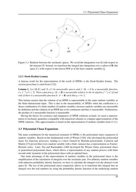
3.3 Polynomial Chaos Expansions Figure 3.1: Relation between the stochastic spaces. We avoid the integration over Ω with respect to the measure Π. Instead, we transform the integral into integration over a subset of IR (the space Γ i ) with respect to the known PDF ρ of the basic random variables ξ i . 3.2.3 Doob-Dynkin Lemma A famous result for the representation of the result of SPDEs is the Doob-Dynkin lemma. The version given here is cited from [132]: Lemma 1. Let (Ω,Σ) and (S,A ) be measurable spaces and f : Ω → S be a measurable function, i.e. f −1 (A ) ⊂ Σ. Then a function g : Ω → IR is measurable relative to the σ-algebra f −1 (A ) if and only if there is a measurable function h : S → IR such that g = h ◦ f . This lemma ensures that the solution of an SPDE is representable in the same random variables as the finite-dimensional input. This is due to the measurability of SPDEs when the coefficient is a linear combination of a finite number of random variables, because random variables are measurable by definition and the solution of an SPDE has to be continuous and thus is measurable. Furthermore, the product of a measurable function is measurable. Having the theory for existence and uniqueness of SPDE solutions at hand, we need a representation of stochastic quantities compatible with numerical schemes to compute approximations of the SPDE solutions. This approximation is based on the representation of random variables from (3.11). 3.3 Polynomial Chaos Expansions The main contribution for the numerical treatment of SPDEs is the polynomial chaos expansion of random variables. Based on the fundamental work of Wiener [156], who developed the polynomial chaos for Gaussian processes, leading to a basis formed by Hermite-polynomials, Cameron and Martin [27] proved that every random variable with a finite variance has a representation as Fourier- Hermite series. Later, Xiu and Karniadakis [160] developed the Wiener-Askey polynomial chaos or generalized polynomial chaos, which allows a representation of any random process with finite second-order moments in the polynomial chaos with an optimal basis. One main advantage of the representation of random variables in the polynomial chaos is the simplification of the calculation of integrals over the stochastic part. For arbitrary random variables with unknown probability density function, we have to calculate the integral over the abstract event space Ω. The use of the polynomial chaos expansions allows us to transform this integral into an integral over the real numbers by using the probability density function of the underlying random 29
Page 1: Segmentation of Stochastic Images u
Page 5: Abstract The task of segmentation,
Page 8 and 9: 7.5 Segmentation of Stochastic Imag
Page 11 and 12: Chapter 1 Introduction The developm
Page 13 and 14: Figure 1.3: This thesis combines fi
Page 15: the presentation of the stochastic
Page 18 and 19: Chapter 2 Image Segmentation and Li
Page 36 and 37: Chapter 3 SPDEs and Polynomial Chao
Page 48 and 49: Chapter 4 Discretization of SPDEs F
Page 50 and 51: Chapter 4 Discretization of SPDEs 4
Page 52 and 53: Chapter 4 Discretization of SPDEs a
Page 58 and 59: Chapter 5 Stochastic Images
Page 60 and 61: Chapter 5 Stochastic Images Figure
Page 62 and 63: Chapter 5 Stochastic Images like qu
Page 64 and 65: Chapter 5 Stochastic Images Figure
Page 67 and 68: Chapter 6 Segmentation of Stochasti
Page 69 and 70: 6.1 Random Walker Segmentation on S
Page 77 and 78: 6.2 Ambrosio-Tortorelli Segmentatio
Page 87: 6.2 Ambrosio-Tortorelli Segmentatio
Page 90 and 91:
Chapter 7 Stochastic Level Sets whe
Page 92 and 93:
Chapter 7 Stochastic Level Sets Fig
Page 94 and 95:
Chapter 7 Stochastic Level Sets and
Page 96 and 97:
Chapter 7 Stochastic Level Sets rar
Page 98 and 99:
Page 100 and 101:
Chapter 7 Stochastic Level Sets MC
Page 102 and 103:
Page 104 and 105:
Page 106 and 107:
Chapter 7 Stochastic Level Sets act
Page 108 and 109:
Chapter 8 Segmentation of Classical
Page 110 and 111:
Page 112 and 113:
Page 114 and 115:
Page 116 and 117:
Page 118 and 119:
Chapter 9 Summary, Discussion, and
Page 121 and 122:
List of Figures 1.1 Left: CT image
Page 123 and 124:
List of Figures 6.2 Mean and varian
Page 125:
List of Figures 7.12 Mean (left) of
Page 129 and 130:
Appendix A Publications Written Dur
Page 131 and 132:
Bibliography [14] L. Ambrosio and M
Page 133 and 134:
Bibliography [46] B. Echebarria, R.
Page 135 and 136:
Bibliography [81] B. N. Khoromskij
Page 137 and 138:
Bibliography [113] A. Nouy. A gener
Page 139:
Bibliography [147] J. Tryoen, O. Le
show all

Segmentation of Stochastic Images using ... - Jacobs University

Create successful ePaper yourself

Delete template?

Save as template?