Segmentation of Stochastic Images using ... - Jacobs University

7.4 Numerical Experiments
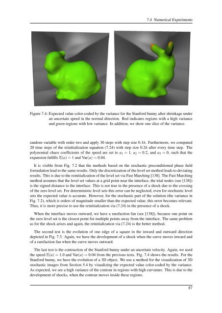
Figure 7.4: Expected value color-coded by the variance for the Stanford bunny after shrinkage under
an uncertain speed in the normal direction. Red indicates regions with a high variance
and green regions with low variance. In addition, we show one slice of the variance.
random variable with order two and apply 30 steps with step size 0.1h. Furthermore, we computed
20 time steps of the reinitialization equation (7.24) with step size 0.2h after every time step. The
polynomial chaos coefficients of the speed are set to a 1 = 1, a 2 = 0.2, and a 3 = 0, such that the
expansion fulfills E(a) = 1 and Var(a) = 0.04.
It is visible from Fig. 7.2 that the methods based on the stochastic preconditioned phase field
formulation lead to the same results. Only the discretization of the level set method leads to deviating
results. This is due to the reinitialization of the level set via Fast Marching [138]. The Fast Marching
method assumes that the level set values at a grid point near the interface, the trial nodes (see [138])
is the signed distance to the interface. This is not true in the presence of a shock due to the crossing
of the zero level set. For deterministic level sets this error can be neglected, even for stochastic level
sets the expected value is accurate. However, for the stochastic part of the solution (the variance in
Fig. 7.2), which is orders of magnitude smaller than the expected value, this error becomes relevant.
Thus, it is more precise to use the reinitialization via (7.24) in the presence of a shock.
When the interface moves outward, we have a rarefaction fan (see [138]), because one point on
the zero level set is the closest point for multiple points away from the interface. The same problem
as for the shock arises and again, the reinitialization via (7.24) is the better method.
The second test is the evolution of one edge of a square in the inward and outward direction
depicted in Fig. 7.3. Again, we have the development of a shock when the curve moves inward and
of a rarefaction fan when the curve moves outward.
The last test is the contraction of the Stanford bunny under an uncertain velocity. Again, we used
the speed E(a) = 1.0 and Var(a) = 0.04 from the previous tests. Fig. 7.4 shows the results. For the
Stanford bunny, we have the evolution of a 3D object. We use a method for the visualization of 3D
stochastic images from Section 5.4 by visualizing the expected value color-coded by the variance.
As expected, we see a high variance of the contour in regions with high curvature. This is due to the
development of shocks, when the contour moves inside these regions.
87