Segmentation of Stochastic Images using ... - Jacobs University

Chapter 6 Segmentation of Stochastic Images Using Elliptic SPDEs
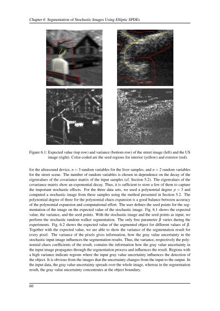
Figure 6.1: Expected value (top row) and variance (bottom row) of the street image (left) and the US
image (right). Color-coded are the seed regions for interior (yellow) and exterior (red).
for the ultrasound device, n = 3 random variables for the liver samples, and n = 2 random variables
for the street scene. The number of random variables is chosen in dependence on the decay of the
eigenvalues of the covariance matrix of the input samples (cf. Section 5.2). The eigenvalues of the
covariance matrix show an exponential decay. Thus, it is sufficient to store a few of them to capture
the important stochastic effects. For the three data sets, we used a polynomial degree p = 3 and
computed a stochastic image from these samples using the method presented in Section 5.2. The
polynomial degree of three for the polynomial chaos expansion is a good balance between accuracy
of the polynomial expansion and computational effort. The user defines the seed points for the segmentation
of the image on the expected value of the stochastic image. Fig. 6.1 shows the expected
value, the variance, and the seed points. With the stochastic image and the seed points as input, we
perform the stochastic random walker segmentation. The only free parameter β varies during the
experiments. Fig. 6.2 shows the expected value of the segmented object for different values of β.
Together with the expected value, we are able to show the variance of the segmentation result for
every pixel. The variance of the pixels gives information, how the gray value uncertainty in the
stochastic input image influences the segmentation results. Thus, the variance, respectively the polynomial
chaos coefficients of the result, contains the information how the gray value uncertainty in
the input image propagates through the segmentation process and influences the result. Regions with
a high variance indicate regions where the input gray value uncertainty influences the detection of
the object. It is obvious from the images that the uncertainty changes from the input to the output. In
the input data, the gray value uncertainty spreads over the whole image, whereas in the segmentation
result, the gray value uncertainty concentrates at the object boundary.
60