Segmentation of Stochastic Images using ... - Jacobs University

6.1 Random Walker Segmentation on Stochastic Images
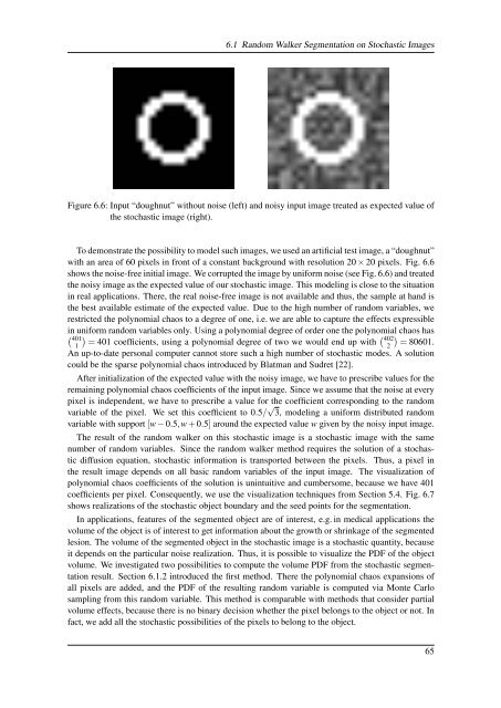
Figure 6.6: Input “doughnut” without noise (left) and noisy input image treated as expected value of
the stochastic image (right).
To demonstrate the possibility to model such images, we used an artificial test image, a “doughnut”
with an area of 60 pixels in front of a constant background with resolution 20 × 20 pixels. Fig. 6.6
shows the noise-free initial image. We corrupted the image by uniform noise (see Fig. 6.6) and treated
the noisy image as the expected value of our stochastic image. This modeling is close to the situation
in real applications. There, the real noise-free image is not available and thus, the sample at hand is
the best available estimate of the expected value. Due to the high number of random variables, we
restricted the polynomial chaos to a degree of one, i.e. we are able to capture the effects expressible
in
(
uniform random variables only. Using a polynomial degree of order one the polynomial chaos has
401
) (
1 = 401 coefficients, using a polynomial degree of two we would end up with 402
)
2 = 80601.
An up-to-date personal computer cannot store such a high number of stochastic modes. A solution
could be the sparse polynomial chaos introduced by Blatman and Sudret [22].
After initialization of the expected value with the noisy image, we have to prescribe values for the
remaining polynomial chaos coefficients of the input image. Since we assume that the noise at every
pixel is independent, we have to prescribe a value for the coefficient corresponding to the random
variable of the pixel. We set this coefficient to 0.5/ √ 3, modeling a uniform distributed random
variable with support [w − 0.5,w + 0.5] around the expected value w given by the noisy input image.
The result of the random walker on this stochastic image is a stochastic image with the same
number of random variables. Since the random walker method requires the solution of a stochastic
diffusion equation, stochastic information is transported between the pixels. Thus, a pixel in
the result image depends on all basic random variables of the input image. The visualization of
polynomial chaos coefficients of the solution is unintuitive and cumbersome, because we have 401
coefficients per pixel. Consequently, we use the visualization techniques from Section 5.4. Fig. 6.7
shows realizations of the stochastic object boundary and the seed points for the segmentation.
In applications, features of the segmented object are of interest, e.g. in medical applications the
volume of the object is of interest to get information about the growth or shrinkage of the segmented
lesion. The volume of the segmented object in the stochastic image is a stochastic quantity, because
it depends on the particular noise realization. Thus, it is possible to visualize the PDF of the object
volume. We investigated two possibilities to compute the volume PDF from the stochastic segmentation
result. Section 6.1.2 introduced the first method. There the polynomial chaos expansions of
all pixels are added, and the PDF of the resulting random variable is computed via Monte Carlo
sampling from this random variable. This method is comparable with methods that consider partial
volume effects, because there is no binary decision whether the pixel belongs to the object or not. In
fact, we add all the stochastic possibilities of the pixels to belong to the object.
65