Segmentation of Stochastic Images using ... - Jacobs University

More documents

Recommendations

Info

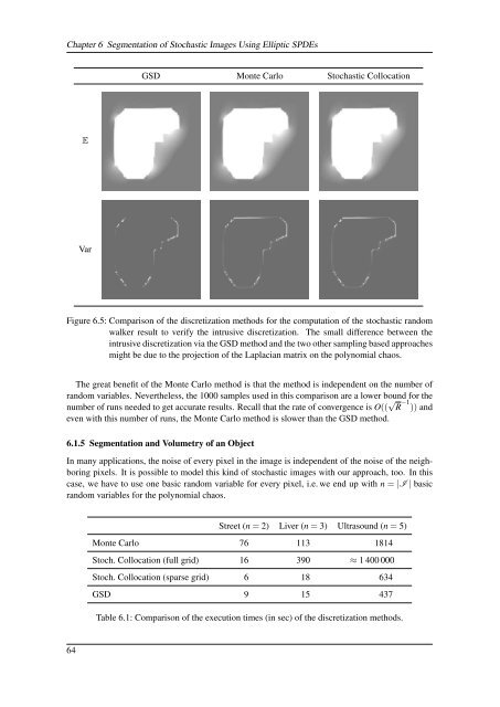
Chapter 6 Segmentation of Stochastic Images Using Elliptic SPDEs GSD Monte Carlo Stochastic Collocation E Var Figure 6.5: Comparison of the discretization methods for the computation of the stochastic random walker result to verify the intrusive discretization. The small difference between the intrusive discretization via the GSD method and the two other sampling based approaches might be due to the projection of the Laplacian matrix on the polynomial chaos. The great benefit of the Monte Carlo method is that the method is independent on the number of random variables. Nevertheless, the 1000 samples used in this comparison are a lower bound for the number of runs needed to get accurate results. Recall that the rate of convergence is O(( √ R −1 )) and even with this number of runs, the Monte Carlo method is slower than the GSD method. 6.1.5 Segmentation and Volumetry of an Object In many applications, the noise of every pixel in the image is independent of the noise of the neighboring pixels. It is possible to model this kind of stochastic images with our approach, too. In this case, we have to use one basic random variable for every pixel, i.e. we end up with n = |I | basic random variables for the polynomial chaos. Street (n = 2) Liver (n = 3) Ultrasound (n = 5) Monte Carlo 76 113 1814 Stoch. Collocation (full grid) 16 390 ≈ 1 400 000 Stoch. Collocation (sparse grid) 6 18 634 GSD 9 15 437 Table 6.1: Comparison of the execution times (in sec) of the discretization methods. 64
6.1 Random Walker Segmentation on Stochastic Images Figure 6.6: Input “doughnut” without noise (left) and noisy input image treated as expected value of the stochastic image (right). To demonstrate the possibility to model such images, we used an artificial test image, a “doughnut” with an area of 60 pixels in front of a constant background with resolution 20 × 20 pixels. Fig. 6.6 shows the noise-free initial image. We corrupted the image by uniform noise (see Fig. 6.6) and treated the noisy image as the expected value of our stochastic image. This modeling is close to the situation in real applications. There, the real noise-free image is not available and thus, the sample at hand is the best available estimate of the expected value. Due to the high number of random variables, we restricted the polynomial chaos to a degree of one, i.e. we are able to capture the effects expressible in ( uniform random variables only. Using a polynomial degree of order one the polynomial chaos has 401 ) ( 1 = 401 coefficients, using a polynomial degree of two we would end up with 402 ) 2 = 80601. An up-to-date personal computer cannot store such a high number of stochastic modes. A solution could be the sparse polynomial chaos introduced by Blatman and Sudret [22]. After initialization of the expected value with the noisy image, we have to prescribe values for the remaining polynomial chaos coefficients of the input image. Since we assume that the noise at every pixel is independent, we have to prescribe a value for the coefficient corresponding to the random variable of the pixel. We set this coefficient to 0.5/ √ 3, modeling a uniform distributed random variable with support [w − 0.5,w + 0.5] around the expected value w given by the noisy input image. The result of the random walker on this stochastic image is a stochastic image with the same number of random variables. Since the random walker method requires the solution of a stochastic diffusion equation, stochastic information is transported between the pixels. Thus, a pixel in the result image depends on all basic random variables of the input image. The visualization of polynomial chaos coefficients of the solution is unintuitive and cumbersome, because we have 401 coefficients per pixel. Consequently, we use the visualization techniques from Section 5.4. Fig. 6.7 shows realizations of the stochastic object boundary and the seed points for the segmentation. In applications, features of the segmented object are of interest, e.g. in medical applications the volume of the object is of interest to get information about the growth or shrinkage of the segmented lesion. The volume of the segmented object in the stochastic image is a stochastic quantity, because it depends on the particular noise realization. Thus, it is possible to visualize the PDF of the object volume. We investigated two possibilities to compute the volume PDF from the stochastic segmentation result. Section 6.1.2 introduced the first method. There the polynomial chaos expansions of all pixels are added, and the PDF of the resulting random variable is computed via Monte Carlo sampling from this random variable. This method is comparable with methods that consider partial volume effects, because there is no binary decision whether the pixel belongs to the object or not. In fact, we add all the stochastic possibilities of the pixels to belong to the object. 65
Page 1:
Segmentation of Stochastic Images u
Page 5:
Abstract The task of segmentation,
Page 8 and 9:
7.5 Segmentation of Stochastic Imag
Page 11 and 12:
Chapter 1 Introduction The developm
Page 13 and 14:
Figure 1.3: This thesis combines fi
Page 15:
the presentation of the stochastic
Page 18 and 19:
Chapter 2 Image Segmentation and Li
Page 20 and 21:
Page 22 and 23:
Page 24 and 25: Chapter 2 Image Segmentation and Li
Page 36 and 37: Chapter 3 SPDEs and Polynomial Chao
Page 48 and 49: Chapter 4 Discretization of SPDEs F
Page 50 and 51: Chapter 4 Discretization of SPDEs 4
Page 52 and 53: Chapter 4 Discretization of SPDEs a
Page 58 and 59: Chapter 5 Stochastic Images
Page 60 and 61: Chapter 5 Stochastic Images Figure
Page 62 and 63: Chapter 5 Stochastic Images like qu
Page 64 and 65: Chapter 5 Stochastic Images Figure
Page 67 and 68: Chapter 6 Segmentation of Stochasti
Page 69 and 70: 6.1 Random Walker Segmentation on S
Page 71 and 72: 6.1 Random Walker Segmentation on S
Page 73: 6.1 Random Walker Segmentation on S
Page 77 and 78: 6.2 Ambrosio-Tortorelli Segmentatio
Page 87: 6.2 Ambrosio-Tortorelli Segmentatio
Page 90 and 91: Chapter 7 Stochastic Level Sets whe
Page 92 and 93: Chapter 7 Stochastic Level Sets Fig
Page 94 and 95: Chapter 7 Stochastic Level Sets and
Page 96 and 97: Chapter 7 Stochastic Level Sets rar
Page 100 and 101: Chapter 7 Stochastic Level Sets MC
Page 106 and 107: Chapter 7 Stochastic Level Sets act
Page 108 and 109: Chapter 8 Segmentation of Classical
Page 118 and 119: Chapter 9 Summary, Discussion, and
Page 121 and 122: List of Figures 1.1 Left: CT image
Page 123 and 124: List of Figures 6.2 Mean and varian
Page 125:
List of Figures 7.12 Mean (left) of
Page 129 and 130:
Appendix A Publications Written Dur
Page 131 and 132:
Bibliography [14] L. Ambrosio and M
Page 133 and 134:
Bibliography [46] B. Echebarria, R.
Page 135 and 136:
Bibliography [81] B. N. Khoromskij
Page 137 and 138:
Bibliography [113] A. Nouy. A gener
Page 139:
Bibliography [147] J. Tryoen, O. Le
show all

Segmentation of Stochastic Images using ... - Jacobs University

You also want an ePaper? Increase the reach of your titles

Delete template?

Save as template?