Segmentation of Stochastic Images using ... - Jacobs University

More documents

Recommendations

Info

Chapter 2 Image Segmentation and Limitations Phase fields are frequently used for interface tracking (see [23, 143] and the references therein), also the image processing community uses phase fields for segmentation purposes [15, 123]. In contrast to the phase field used in the Ambrosio-Tortorelli approach, the phase fields needed in this context differentiate between object and background, i.e. they describe closed contours. They have a value of −1 in the object, 0 at the interface, +1 on the background and vary smoothly between these values. Typically, the phase field is ±1 away from the interface and changes smoothly inside a small layer with thickness ε around the interface in a tangential profile. A phase field equation [143] like ( φ t + F|∇φ| + u e · ∇φ = b ∆φ + φ(1 − φ 2 ) ) ε 2 (2.31) controls the evolution of the diffusive phase field interface. In this equation, φ is the phase field, u e an external advection, b the interface speed depending on the curvature, ε the thickness of the diffusive interface, and F again the speed in the normal direction. In contrast to the level set approach (2.30), this is a parabolic equation, which avoids the numerical difficulties arising in the discretization of the level set equation. When the curvature-depending interface speed vanishes, i.e. when b = 0, this equation is kept parabolic by adding a counter term introduced by Folch [51]. Following [143] this counter term leads to the parabolic equation ( φ t + F|∇φ| + u e · ∇φ = b ∆φ + φ(1 − φ 2 ( )) ) ∇φ ε 2 − |∇φ|∇ · , (2.32) |∇φ| where b is a purely numerical parameter, because the curvature at the end cancels out the Laplacian and the term φ(1−φ 2 ) . It is easier to discretize (2.32) than (2.30) using central differences. Sun et ε 2 al. [143] developed a phase field equation based on nonlinear preconditioning [56] ( φ t + a|∇φ| + u e · ∇φ = b ∆φ + 1 ε (1 − |∇φ|2 ) √ ( ) ( )) φ ∇φ 2tanh √ − |∇φ|∇ · , (2.33) 2ε |∇φ| which is an integrated reinitialization scheme for the phase field. The phase field φ in this equation becomes a signed distance function. Thus, this equation is a parabolic level set equation with integrated reinitialization. Again, it is possible to discretize (2.33) using simple difference schemes. This connection between phase fields and level sets allows us to use known segmentation algorithms from the level set context and embed them into this nonlinear preconditioned phase field equation. The discretization of the parabolic phase field equations is easier in the stochastic context, cf. Chapter 7. 2.4.2 Gradient-Based Segmentation The idea of the level set propagation is useful to segment objects inside an image. The simplest approach for segmentation based on level sets is to use a speed F in the level set equation that depends on characteristics of the image. Popular is F = F(|∇u|), i.e. to stop the evolution on edges inside the image (see [29, 96, 138] and the references therein). Caselles et al. [29] proposed to use with g u = φ t + g u |∇φ| = 0 (2.34) 1 (1 − εκ) , (2.35) 1 + |∇G σ ∗ u| where u is the image, G σ a Gaussian smoothing filter with width σ, κ the curvature of the level set function and ε a small scale parameter that controls the influence of the curvature smoothing term. Although this idea sounds simple, the method achieves good results when a high gradient separates the objects from the background (see Fig. 2.7). One major drawback of this method is the need for 18
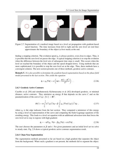
2.4 Level Sets for Image Segmentation Figure 2.7: Segmentation of a medical image based on a level set propagation with gradient-based speed function. The time increases from left to right and the zero level set (red line) approximates the boundary of the object (a liver mask) at the end. finding a stopping criterion. The evolution speed g u is always positive, even close to edges. Thus, it is possible that the zero level set passes the edge. A typical stopping criterion is to stop the evolution when the difference between the level sets of subsequent time steps is small. This occurs when the level set reached the boundary of the object and the speed dropped down. Using methods that are more sophisticated, it is possible to stop the zero level set at the edge. Thus, these methods have a convergent solution. The next section presents one of these methods, geodesic active contours. Remark 5. It is also possible to formulate the gradient-based segmentation based on the phase field model presented in the last section. This yields the equation ( φ t + g u |∇φ| = ε ∆φ + φ(1 − φ 2 ) ) ε 2 . (2.36) 2.4.3 Geodesic Active Contours Caselles et al. [30] and simultaneously Kichenassamy et al. [82] developed geodesic, or minimal distance, active contours. They minimize an energy B that depends on the curve C and on the parametrization of the curve C(q) : [0,1] → IR 2 : ∫ 1 B(C) = α |C ′ (q)| 2 dq + β 0 ∫ 1 0 g u (|∇u(C(q))|) 2 dq , (2.37) where g u is the edge indicator from the last section. They computed a minimizer of this energy by using a level set representation of the curve and computing the Euler-Lagrange equations of the resulting energy. This leads to a level set equation with an additional advection term that forces the zero level set to stay in regions with high gradient: φ t = −α∇g u · ∇φ − βg u |∇φ| + εκ|∇φ| . (2.38) The user chooses the parameters α,β and ε. For given parameters and an initial level set we solve to steady state. Fig. 2.8 shows a typical geodesic active contours segmentation result. 2.4.4 Chan-Vese Segmentation The segmentation methods presented so far are based on a high gradient that separates the object from the background. When such a gradient is not present, the methods fail to segment the object. 19
Page 1: Segmentation of Stochastic Images u
Page 5: Abstract The task of segmentation,
Page 8 and 9: 7.5 Segmentation of Stochastic Imag
Page 11 and 12: Chapter 1 Introduction The developm
Page 13 and 14: Figure 1.3: This thesis combines fi
Page 15: the presentation of the stochastic
Page 18 and 19: Chapter 2 Image Segmentation and Li
Page 36 and 37: Chapter 3 SPDEs and Polynomial Chao
Page 48 and 49: Chapter 4 Discretization of SPDEs F
Page 50 and 51: Chapter 4 Discretization of SPDEs 4
Page 52 and 53: Chapter 4 Discretization of SPDEs a
Page 58 and 59: Chapter 5 Stochastic Images
Page 60 and 61: Chapter 5 Stochastic Images Figure
Page 62 and 63: Chapter 5 Stochastic Images like qu
Page 64 and 65: Chapter 5 Stochastic Images Figure
Page 67 and 68: Chapter 6 Segmentation of Stochasti
Page 69 and 70: 6.1 Random Walker Segmentation on S
Page 77 and 78: 6.2 Ambrosio-Tortorelli Segmentatio
Page 79 and 80:
6.2 Ambrosio-Tortorelli Segmentatio
Page 81 and 82:
Page 83 and 84:
Page 85 and 86:
Page 87:
Page 90 and 91:
Chapter 7 Stochastic Level Sets whe
Page 92 and 93:
Chapter 7 Stochastic Level Sets Fig
Page 94 and 95:
Chapter 7 Stochastic Level Sets and
Page 96 and 97:
Chapter 7 Stochastic Level Sets rar
Page 98 and 99:
Page 100 and 101:
Chapter 7 Stochastic Level Sets MC
Page 102 and 103:
Page 104 and 105:
Page 106 and 107:
Chapter 7 Stochastic Level Sets act
Page 108 and 109:
Chapter 8 Segmentation of Classical
Page 110 and 111:
Page 112 and 113:
Page 114 and 115:
Page 116 and 117:
Page 118 and 119:
Chapter 9 Summary, Discussion, and
Page 121 and 122:
List of Figures 1.1 Left: CT image
Page 123 and 124:
List of Figures 6.2 Mean and varian
Page 125:
List of Figures 7.12 Mean (left) of
Page 129 and 130:
Appendix A Publications Written Dur
Page 131 and 132:
Bibliography [14] L. Ambrosio and M
Page 133 and 134:
Bibliography [46] B. Echebarria, R.
Page 135 and 136:
Bibliography [81] B. N. Khoromskij
Page 137 and 138:
Bibliography [113] A. Nouy. A gener
Page 139:
Bibliography [147] J. Tryoen, O. Le
show all

Segmentation of Stochastic Images using ... - Jacobs University

You also want an ePaper? Increase the reach of your titles

Delete template?

Save as template?