Segmentation of Stochastic Images using ... - Jacobs University

More documents

Recommendations

Info

Chapter 7 Stochastic Level Sets Figure 7.9: Left: Evolution of the expected value contour of the stochastic geodesic active contour method. The shown variance corresponds to the contour after 240 iterations (the magenta contour). Right: Mean value of the stochastic image to be segmented and the contours at time points of the level set evolution. The final contour matches the object boundary. Numerical Results The application of the stochastic geodesic active contour method is demonstrated on the same data sets as the gradient-based segmentation on stochastic images, namely the stochastic CT image and the liver mask with two random variables and a polynomial degree of two. A comparison of the intrusive implementation using the polynomial chaos expansion and the sampling based implementations using Monte Carlo simulation and stochastic collocation is depicted in Fig. 7.8 for the CT data and shows a good consistency of the implementations. Fig. 7.9 shows the expected value contour for time points during the level set evolution together with the variance of the final level set of the segmentation of the second data set. Again, the regions with a high variance are the bottom and the upper-right side of the object. This is consistent with the results from the gradient-based segmentation (cf. Fig. 7.6). Furthermore, the right picture of Fig. 7.9 shows the evolution of the expected value contour on the expected value image. The expected value contour after 240 iterations with a time step of 0.2h is aligned to the object boundary. The variance corresponding to this contour is the same as the variance in the left picture of the same figure. The advantage of the stochastic geodesic active contour approach over the stochastic gradientbased segmentation is that a running over the edges is mostly avoided (cf. Fig. 7.11). 7.5.3 Stochastic Chan-Vese segmentation We derive the stochastic Chan-Vese model from classical Chan-Vese model by replacing all quantities by their stochastic counterparts: ( ( ) ) ∇φ φ t = δ ε (φ) µ∇ · − ν − λ 1 (u 0 − c 1 ) 2 + λ 2 (u 0 − c 2 ) 2 |∇φ| , (7.36) where the phase field φ, the initial image u 0 , the mean values c 1 and c 2 , and the smooth delta approximation δ ε are stochastic quantities, i.e. they are dependent on the random event ω ∈ Ω. The function δ ε is the derivative of the stochastic smooth Heaviside approximation H ε (z(ω)) = 1 2 ( 1 + 2 ( )) z(ω) π arctan ε . (7.37) 92
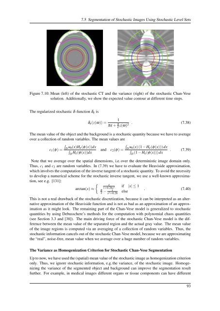
7.5 Segmentation of Stochastic Images Using Stochastic Level Sets Figure 7.10: Mean (left) of the stochastic CT and the variance (right) of the stochastic Chan-Vese solution. Additionally, we show the expected value contour at different time steps. The regularized stochastic δ-function δ ε is 1 δ ε (z(ω)) = πε + π . (7.38) ε z(ω)2 The mean value of the object and the background is a stochastic quantity because we have to average over a collection of random variables. The mean values are ∫ D c 1 (φ) = u ∫ 0(x)H ε (φ(x))dx ∫ D D H and c 2 (φ) = u 0(x)(1 − H ε (φ(x)))dx ∫ ε(φ(x))dx D (1 − H . (7.39) ε(φ(x)))dx Note that we average over the spatial dimensions, i.e. over the deterministic image domain only. Thus, c 1 and c 2 are random variables. In (7.39) we have to evaluate the Heaviside approximation, which involves the computation of the inverse tangent of a stochastic quantity. To avoid the necessity to develop a numerical scheme for the stochastic inverse tangent, we use a well-known approximation, see e.g. [131]: { x arctan(x) ≈ 1+0.28x 2 if |x| ≤ 1 else π 2 − x x 2 +0.28 . (7.40) This is not a real drawback of the stochastic discretization, because it can be interpreted as an alternative approximation of the Heaviside function and is not as bad as an approximation of an approximation as it might look. The remaining part of the Chan-Vese model is generalized to stochastic quantities by using Debusschere’s methods for the computation with polynomial chaos quantities (see Section 3.3 and [38]). The main driving force of the stochastic Chan-Vese model is the difference between the mean value of the separated region and the actual gray value. The mean value of the image regions is computed via an averaging of a collection of random variables. Thus, the stochastic information cancels out of the stochastic Chan-Vese model, because we are approximating the “real”, noise-free, mean value when we average over a huge number of random variables. The Variance as Homogenization Criterion for Stochastic Chan-Vese Segmentation Up to now, we have used the (spatial) mean value of the stochastic image as homogenization criterion only. Thus, we ignore stochastic information, e.g. the variance, of the stochastic image. Homogenizing the variance of the segmented object and background can improve the segmentation result further. For example, in medical images different organs or tissue components can have different 93
Page 1:
Segmentation of Stochastic Images u
Page 5:
Abstract The task of segmentation,
Page 8 and 9:
7.5 Segmentation of Stochastic Imag
Page 11 and 12:
Chapter 1 Introduction The developm
Page 13 and 14:
Figure 1.3: This thesis combines fi
Page 15:
the presentation of the stochastic
Page 18 and 19:
Chapter 2 Image Segmentation and Li
Page 20 and 21:
Page 22 and 23:
Page 24 and 25:
Page 26 and 27:
Page 28 and 29:
Page 30 and 31:
Page 32 and 33:
Page 34 and 35:
Page 36 and 37:
Chapter 3 SPDEs and Polynomial Chao
Page 38 and 39:
Page 40 and 41:
Page 42 and 43:
Page 44 and 45:
Page 46 and 47:
Page 48 and 49:
Chapter 4 Discretization of SPDEs F
Page 50 and 51:
Chapter 4 Discretization of SPDEs 4
Page 52 and 53: Chapter 4 Discretization of SPDEs a
Page 54 and 55: Chapter 4 Discretization of SPDEs F
Page 56 and 57: Chapter 4 Discretization of SPDEs F
Page 58 and 59: Chapter 5 Stochastic Images
Page 60 and 61: Chapter 5 Stochastic Images Figure
Page 62 and 63: Chapter 5 Stochastic Images like qu
Page 64 and 65: Chapter 5 Stochastic Images Figure
Page 67 and 68: Chapter 6 Segmentation of Stochasti
Page 69 and 70: 6.1 Random Walker Segmentation on S
Page 77 and 78: 6.2 Ambrosio-Tortorelli Segmentatio
Page 87: 6.2 Ambrosio-Tortorelli Segmentatio
Page 90 and 91: Chapter 7 Stochastic Level Sets whe
Page 92 and 93: Chapter 7 Stochastic Level Sets Fig
Page 94 and 95: Chapter 7 Stochastic Level Sets and
Page 96 and 97: Chapter 7 Stochastic Level Sets rar
Page 100 and 101: Chapter 7 Stochastic Level Sets MC
Page 106 and 107: Chapter 7 Stochastic Level Sets act
Page 108 and 109: Chapter 8 Segmentation of Classical
Page 118 and 119: Chapter 9 Summary, Discussion, and
Page 121 and 122: List of Figures 1.1 Left: CT image
Page 123 and 124: List of Figures 6.2 Mean and varian
Page 125: List of Figures 7.12 Mean (left) of
Page 129 and 130: Appendix A Publications Written Dur
Page 131 and 132: Bibliography [14] L. Ambrosio and M
Page 133 and 134: Bibliography [46] B. Echebarria, R.
Page 135 and 136: Bibliography [81] B. N. Khoromskij
Page 137 and 138: Bibliography [113] A. Nouy. A gener
Page 139: Bibliography [147] J. Tryoen, O. Le
show all

Segmentation of Stochastic Images using ... - Jacobs University

Create successful ePaper yourself

Delete template?

Save as template?