Segmentation of Stochastic Images using ... - Jacobs University

More documents

Recommendations

Info

Chapter 7 Stochastic Level Sets Figure 7.5: Mean of the CT data set (left) and the liver data set (right) for the segmentation test. 7.5 Segmentation of Stochastic Images Using Stochastic Level Sets Level set evolution with an uncertain speed can be useful in applications, e.g. in physical applications where level sets track the interface between materials. Often, the material parameters are not known exactly and the interface speed can be modeled dependent on the random material parameters. The focus of this thesis is on the application of segmentation methods. This is why we use this new concept for stochastic level sets at the moment for segmentation only. The author used level sets for the modeling of physical effects, the evaporation of water during radiofrequency ablation [10,11,13]. It is possible to use stochastic level sets in this context, because the material parameters can be modeled as random variables [87, 128] which leads to an uncertain interface speed. For segmentation, we investigate three segmentation methods based on level sets for stochastic extensions: gradient-based segmentation, geodesic active contours, and Chan-Vese segmentation. Other segmentation methods based on level sets can also be suitable for stochastic extensions. 7.5.1 Gradient-Based Segmentation of Stochastic Images Gradient-based segmentation of an image u : D → IR is introduced in Section 2.4.2 and given by φ t + v(1 − bκ)|∇φ| = 0 , (7.26) where the function v is called stopping function, because this function controls the stopping of the level set evolution at the desired boundaries. Often, the function v is given by v = 1/(1 + |∇u|) , (7.27) where u is the image to segment. Typically, the level set is initialized as the signed distance function of a small circle inside the object to segment. There is no theoretical justification of this method besides the observation that the level set speed is close to zero at sharp edges due to the reciprocal dependence between image gradient and speed. We replace the classical image u(x) by a stochastic image u(x,ω). The equation for stochastic gradient-based segmentation is and the speed is a stochastic quantity, too: φ t (t,x,ω) + v(t,x,ω)(1 − bκ(t,x,ω))|∇φ(t,x,ω)| = 0 (7.28) v(t,x,ω) = 1 1 + |∇u(t,x,ω)| . (7.29) 88
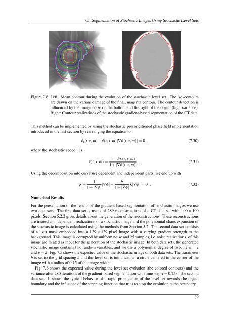
7.5 Segmentation of Stochastic Images Using Stochastic Level Sets Figure 7.6: Left: Mean contour during the evolution of the stochastic level set. The iso-contours are drawn on the variance image of the final, magenta contour. The contour detection is influenced by the image noise on the bottom and the right of the object (high variance). Right: Contour realizations of the stochastic gradient-based segmentation of the CT data. This method can be implemented by using the stochastic preconditioned phase field implementation introduced in the last section by rearranging the equation to where the stochastic speed ṽ is φ t (t,x,ω) + ṽ(t,x,ω)|∇φ(t,x,ω)| = 0 , (7.30) ṽ(t,x,ω) = 1 − bκ(t,x,ω) 1 + |∇φ(t,x,ω)| . (7.31) Using the decomposition into curvature dependent and independent parts, we end up with Numerical Results φ t + 1 1 + |∇φ| |∇φ| − b κ|∇φ| = 0 . (7.32) 1 + |∇φ| For the presentation of the results of the gradient-based segmentation of stochastic images we use two data sets. The first data set consists of 289 reconstructions of a CT data set with 100 × 100 pixels. Section 5.2.2 gives details about the generation of the reconstructions. These reconstructions are treated as independent realizations of a stochastic image and the polynomial chaos expansion of the stochastic image is calculated using the methods from Section 5.2. The second data set consists of a liver mask embedded into a 129 × 129 pixel image with a varying gradient strength to the background. This image is corrupted by uniform noise and 25 samples, i.e. noise realizations, of this image are treated as input for the generation of the stochastic image. In both data sets, the generated stochastic image contains two random variables, and we use a polynomial degree of two, i.e. n = 2 and p = 2. Fig. 7.5 shows the expected value of the stochastic image of both data sets. The parameter b is set to the grid spacing h and the level set is initialized as a circle centered in the center of the image with a radius of 0.15 of the image width. Fig. 7.6 shows the expected value during the level set evolution (the colored contours) and the variance after 280 iterations of the gradient-based segmentation with time step τ = 0.2h of the second data set. It shows the typical behavior of a rapid propagation of the level set towards the object boundary and the influence of the stopping function that tries to stop the evolution at the boundary. 89
Page 1:
Segmentation of Stochastic Images u
Page 5:
Abstract The task of segmentation,
Page 8 and 9:
7.5 Segmentation of Stochastic Imag
Page 11 and 12:
Chapter 1 Introduction The developm
Page 13 and 14:
Figure 1.3: This thesis combines fi
Page 15:
the presentation of the stochastic
Page 18 and 19:
Chapter 2 Image Segmentation and Li
Page 20 and 21:
Page 22 and 23:
Page 24 and 25:
Page 26 and 27:
Page 28 and 29:
Page 30 and 31:
Page 32 and 33:
Page 34 and 35:
Page 36 and 37:
Chapter 3 SPDEs and Polynomial Chao
Page 38 and 39:
Page 40 and 41:
Page 42 and 43:
Page 44 and 45:
Page 46 and 47:
Page 48 and 49: Chapter 4 Discretization of SPDEs F
Page 50 and 51: Chapter 4 Discretization of SPDEs 4
Page 52 and 53: Chapter 4 Discretization of SPDEs a
Page 58 and 59: Chapter 5 Stochastic Images
Page 60 and 61: Chapter 5 Stochastic Images Figure
Page 62 and 63: Chapter 5 Stochastic Images like qu
Page 64 and 65: Chapter 5 Stochastic Images Figure
Page 67 and 68: Chapter 6 Segmentation of Stochasti
Page 69 and 70: 6.1 Random Walker Segmentation on S
Page 77 and 78: 6.2 Ambrosio-Tortorelli Segmentatio
Page 87: 6.2 Ambrosio-Tortorelli Segmentatio
Page 90 and 91: Chapter 7 Stochastic Level Sets whe
Page 92 and 93: Chapter 7 Stochastic Level Sets Fig
Page 94 and 95: Chapter 7 Stochastic Level Sets and
Page 96 and 97: Chapter 7 Stochastic Level Sets rar
Page 100 and 101: Chapter 7 Stochastic Level Sets MC
Page 106 and 107: Chapter 7 Stochastic Level Sets act
Page 108 and 109: Chapter 8 Segmentation of Classical
Page 118 and 119: Chapter 9 Summary, Discussion, and
Page 121 and 122: List of Figures 1.1 Left: CT image
Page 123 and 124: List of Figures 6.2 Mean and varian
Page 125: List of Figures 7.12 Mean (left) of
Page 129 and 130: Appendix A Publications Written Dur
Page 131 and 132: Bibliography [14] L. Ambrosio and M
Page 133 and 134: Bibliography [46] B. Echebarria, R.
Page 135 and 136: Bibliography [81] B. N. Khoromskij
Page 137 and 138: Bibliography [113] A. Nouy. A gener
Page 139: Bibliography [147] J. Tryoen, O. Le
show all

Segmentation of Stochastic Images using ... - Jacobs University

Create successful ePaper yourself

Delete template?

Save as template?