Segmentation of Stochastic Images using ... - Jacobs University

2.3 Mumford-Shah and Ambrosio-Tortorelli Segmentation
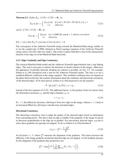
Theorem 2.1. Define Ẽ AT : L 1 (D) × L 1 (D) → IR + by
{
EAT (u,φ) if (u,φ) ∈ H
Ẽ AT (u,φ) :=
1 (D) × H 1 (D),0 ≤ φ ≤ 1
+∞ otherwise
(2.21)
and G : L 1 (D) × L 1 (D) → IR + by
{
EMS (u) if u ∈ GSBV(D) and φ = 1 almost everywhere
G(u,φ) =
+∞ otherwise.
(2.22)
If k ε = o(ε), then Ẽ AT Γ-converges to G(u,φ) for ε → 0.
The convergence of the Ambrosio-Tortorelli energy towards the Mumford-Shah energy enables us
to use the coupled pair of PDEs obtained as Euler-Lagrange equations of the Ambrosio-Tortorelli
energy and to solve this with very small ε. The result is a phase field that is close to the characteristic
function of the edge set of the Mumford-Shah functional.
2.3.3 Edge Continuity and Edge Consistency
The classical Mumford-Shah model and the Ambrosio-Tortorelli approximation lack a step linking
edges. This step is necessary to enforce the detection of closed contours in the images. Otherwise,
the appearance of partially detected, breaking up contours is possible, see Fig. 2.5. For example,
Erdem et al. [49] introduced such a step for the Ambrosio-Tortorelli model. The idea is to use a
modified diffusion coefficient in the image equation. This modified coefficient does not depend on
the phase field exclusively, but contains information about the continuity and directional consistency
of the detected edges. To be more precise, Erdem et al. [49] proposed to use the equation
−∇ · (µ((cφ) 2 + k ε )∇u ) + u = u 0 , (2.23)
instead of the first equation of (2.18). The additional factor c is the product of the two factors from
the directional consistency c dc and the edge continuity c h , i.e.
c = c dc · c h . (2.24)
If c < 1, the diffusivity decreases, allowing to form new edges in the image, whereas c > 1 leads to
an increased diffusivity, allowing to smooth away unwanted edges.
Directional Consistency
The directional consistency tries to judge the quality of the detected edges based on information
from surrounding pixels. The idea is that an edge is reliable if the gradients of the image for pixels
in directions perpendicular to the edge are in parallel. For inaccurately detected edges, e.g. due to
noise, these gradients are typically not aligned. To do so, Erdem et al. [49] introduced
(c dc ) i = ζ dc
i
+ 1 − ζ i
dc
(2.25)
φ i
for all pixels i ∈ I , where ζi
dc measures the alignment of the gradients. This factor increases the
diffusion, if the image gradients around the detected edge are not aligned. As the feedback measure
for the alignment of the gradients they proposed to use
( ( ))
1
ζi
dc = exp ε dc |η s | ∑ ∇v
j∈η s i · ∇v j − 1 , (2.26)
15